Thermodynamics and statistical physics

Guidelines and control tasks for distance learning students

Shelkunova Z.V., Saneev E.L.

Methodological instructions and control tasks for students of distance learning engineering and technological specialties. They contain sections of the programs "Statistical Physics", "Thermodynamics", examples of solving typical problems and options for control tasks.

Keywords: Internal energy, warmth, work; isoprocesses, entropy: distribution functions: Maxwell, Boltzmann, Bose - Einstein; Fermi - Dirac; Fermi energy, heat capacity, Einstein and Debye characteristic temperature.

Editor T.Yu.Artyunina

Prepared for printing d. Format 6080 1/16

R.l. ; uch.-ed.l. 3.0; Circulation ____ copies. Order no.

___________________________________________________

RIO ESGTU, Ulan-Ude, Klyuchevskaya, 40a

Printed on the rotaprint of ESGTU, Ulan-Ude,

Klyuchevskaya, 42.

Federal Agency for Education

East Siberian State

University of Technology

PHYSICS №4

(Thermodynamics and statistical physics)

Methodical instructions and control tasks

for distance learning students

Compiled by: Shelkunova Z.V.

Saneev E.L.

Publishing house of ESGTU

Ulan-Ude, 2009

Statistical physics and thermodynamics

Topic 1

Dynamic and statistical laws in physics. Thermodynamic and statistical methods. Elements of molecular-kinetic theory. macroscopic state. Physical quantities and states of physical systems. Macroscopic parameters as mean values. Thermal balance. Ideal gas model. The equation of state for an ideal gas. The concept of temperature.

Theme 2

transfer phenomena. Diffusion. Thermal conductivity. diffusion coefficient. Coefficient of thermal conductivity. thermal diffusivity. Diffusion in gases, liquids and solids. Viscosity. Viscosity coefficient of gases and liquids.

Theme 3

Elements of thermodynamics. First law of thermodynamics. Internal energy. Intensive and extensive parameters.

Theme 4

Reversible and irreversible processes. Entropy. The second law of thermodynamics. Thermodynamic potentials and equilibrium conditions. chemical potential. Conditions of chemical equilibrium. Carnot cycle.

Theme 5

distribution functions. microscopic parameters. Probability and fluctuations. Maxwell distribution. Medium kinetic energy particles. Boltzmann distribution. Heat capacity of polyatomic gases. Limitation of the classical theory of heat capacity.

Theme 6

Gibbs distribution. Model of the system in the thermostat. Canonical Gibbs distribution. Statistical meaning of thermodynamic potentials and temperature. The role of free energy.

Theme 7

Gibbs distribution for a system with a variable number of particles. Entropy and probability. Determination of the entropy of an equilibrium system through the statistical weight of a microstate.

Theme 8

Bose and Fermi distribution functions. Planck's formula for weightless thermal radiation. Order and disorder in nature. Entropy as a quantitative measure of chaos. The principle of increasing entropy. The transition from order to disorder is about the state of thermal equilibrium.

Theme 9

Experimental methods for studying the vibrational spectrum of crystals. The concept of phonons. Dispersion laws for acoustic and optical phonons. Heat capacity of crystals at low and high temperatures. Electronic heat capacity and thermal conductivity.

Theme 10

Electrons in crystals. Approximation of strong and weak coupling. Model of free electrons. Fermi level. Elements of the band theory of crystals. Bloch function. Band structure of the energy spectrum of electrons.

Topic 11

Fermi surface. The number and density of the number of electronic states in the band. Zone fillings: metals, dielectrics and semiconductors. Electrical conductivity of semiconductors. The concept of hole conductivity. Intrinsic and extrinsic semiconductors. The concept of p-n junction. Transistor.

Theme 12

Electrical conductivity of metals. Current carriers in metals. Insufficiency of classical electron theory. Electronic Fermi gas in a metal. Current carriers as quasiparticles. The phenomenon of superconductivity. Cooper pairing of electrons. tunnel contact. The Josephson effect and its applications. Capture and quantization magnetic flux. The concept of high-temperature conductivity.

STATISTICAL PHYSICS. THERMODYNAMICS

Basic formulas

1. Amount of substance of a homogeneous gas (in moles):

where N-number of gas molecules; N A- Avogadro's number; m-mass of gas;  is the molar mass of the gas.

If the system is a mixture of several gases, then the amount of substance in the system

where  i , N i , m i ,  i - respectively the amount of substance, number of molecules, mass, molar mass i th component of the mixture.

2. Clapeyron-Mendeleev equation (ideal gas equation of state):

where m- mass of gas;  - molar mass; R- universal gas constant;  = m/ - amount of substance; T is the thermodynamic temperature in Kelvin.

3. Experimental gas laws, which are special cases of the Clapeyron-Mendeleev equation for isoprocesses:

boyle-mariotte law

(isothermal process - T= const; m=const):

or for two gas states:

where p 1 and V 1 - pressure and volume of gas in the initial state; p 2 and V 2

Gay-Lussac's law (isobaric process - p=const, m=const):

or for two states:

where V 1 and T 1 - the volume and temperature of the gas in the initial state; V 2 and T 2 - the same values in the final state;

Charles' law (isochoric process - V=const, m=const):

or for two states:

where R 1 and T 1 - pressure and temperature of the gas in the initial state; R 2 and T 2 - the same values in the final state;

combined gas law (m=const):

where R 1 , V 1 , T 1 - pressure, volume and temperature of the gas in the initial state; R 2 , V 2 , T 2 are the same values in the final state.

4. Dalton's law, which determines the pressure of a mixture of gases:

p = p 1 + p 2 + ... +p n

where p i - partial pressures mixture component; n- the number of components of the mixture.

5. Molar mass of a mixture of gases:

where m i- weight i-th component of the mixture;  i = m i / i- amount of substance i-th component of the mixture; n- the number of components of the mixture.

6. Mass fraction  i i-th component of the gas mixture (in fractions of a unit or percentage):

where m is the mass of the mixture.

7. Concentration of molecules (number of molecules per unit volume):

where N-number of molecules contained in the system;  is the density of the substance. The formula is valid not only for gases, but also for any state of aggregation of matter.

8. Basic equation kinetic theory gases:

where<>is the average kinetic energy of the translational motion of the molecule.

9. Average kinetic energy of translational motion of a molecule:

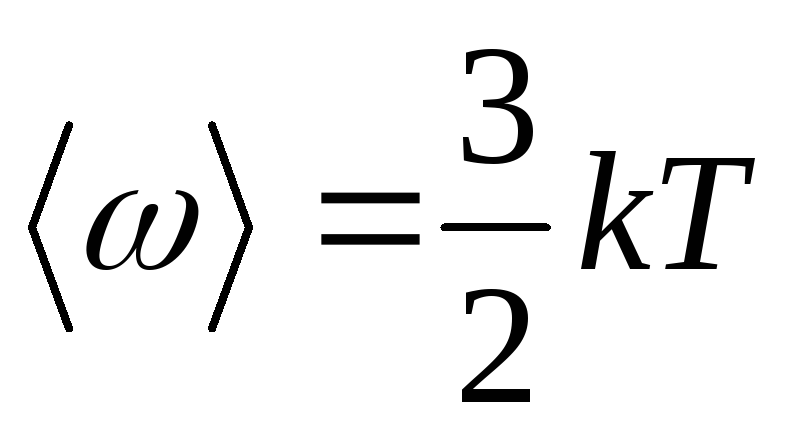where k is the Boltzmann constant.

10. Average total kinetic energy of a molecule:

where i is the number of degrees of freedom of the molecule.

11. Dependence of gas pressure on the concentration of molecules and temperature:

p = nkT.

12. Speeds of molecules:

root mean square ;

arithmetic mean ;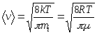

most likely ,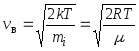

where m i is the mass of one molecule.

13. Relative speed of a molecule:

u = v/v in ,

where v is the speed of this molecule.

14. Specific heat capacities of gas at constant volume (s v) and at constant pressure (With R):

15. Relationship between specific ( With) and molar ( FROM) heat capacities:

; C=c .

16. Robert Mayer Equation:

C p -C v = R.

17. Internal energy of an ideal gas:

18. First law of thermodynamics:

where  Q- heat communicated to the system (gas); dU- change in the internal energy of the system;  BUT is the work done by the system against external forces.

19. Gas expansion work:

in general ;

in isobaric process ;

isothermal process ;

in an adiabatic process ,

or ,

where is the adiabatic exponent.

20. Poisson's equations relating the parameters of an ideal gas in an adiabatic process:

;

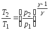21. Thermal efficiency cycle.

electrons, etc.), through the properties of these particles and the interaction between them.

Other branches of physics are also studying macroscopic bodies - thermodynamics , Mechanics continuous media, electrodynamics of continuous media. However, when solving specific problems by the methods of these disciplines, the corresponding equations always include unknown parameters or functions that characterize a given body. So, to solve problems of hydrodynamics, it is necessary to know the equation of state of a liquid or gas, i.e., the dependence of density on temperature and pressure, the heat capacity of a liquid, its viscosity coefficient, etc. All these dependences and parameters can, of course, be determined experimentally; therefore, the methods in question are called phenomenological. Statistical physics allows, at least in principle, and in many cases actually, to calculate all these quantities, if the forces of interaction between molecules are known. That., statistical physics uses information about the "microscopic" structure of bodies - about what particles they consist of, how these particles interact, therefore it is called the microscopic theory.

If at some point in time the coordinates and velocities of all particles of the body are given and the law of their interaction is known, then, by solving the equations of mechanics, it would be possible to find these coordinates and velocities at any subsequent point in time and thereby completely determine the state of the body under study. (For simplicity, the presentation is carried out in the language of classical mechanics. But even in quantum mechanics the situation is the same: knowing the initial wave function systems and the law of interaction of particles, it is possible, by solving Schrödinger equation , find the wave function that determines the state of the system at all future moments of time.) In fact, however, such a way of constructing a microscopic theory is impossible, since the number of particles in macroscopic bodies is very large. For example, in 1 cm 3 gas at a temperature of 0 °C and a pressure of 1 atm contains approximately 2.7×10 19 molecules. It is impossible to solve such a number of equations, and the initial coordinates and velocities of all molecules are still unknown.

However, it big number particles in macroscopic bodies leads to the emergence of new - statistical - regularities in the behavior of such bodies. This behavior in a wide range does not depend on the specific initial conditions - on the exact values of the initial coordinates and particle velocities. The most important manifestation of this independence is the fact known from experience that a system, left to itself, i.e., isolated from external influences, eventually comes to some equilibrium state (thermodynamic, or statistical, equilibrium), the properties of which are determined only by such general characteristics initial state, as the number of particles, their total energy, etc. (cm. Thermodynamic equilibrium ). In what follows, we will focus mainly on statistical physics equilibrium states.

Before formulating a theory that describes statistical regularities, one should reasonably limit the very requirements for the theory. Namely, the task of the theory should be to calculate not the exact values of various physical quantities for macroscopic bodies, but the average values of these quantities over time. Consider, for example, molecules located in a sufficiently large macroscopic volume isolated in a gas. The number of such molecules will change over time due to their movement, and it could be found exactly if all the coordinates of the molecules at all times were known. This, however, is not necessary. The change in the number of molecules in the volume will be in the nature of random fluctuations - fluctuations - relative to some average value. With a large number of particles in the volume, these fluctuations will be small compared to the average number of particles, so that to characterize the macroscopic state, it is sufficient to know just this average value.

To clarify the nature of statistical patterns, consider another simple example. Let a large number of grains of two varieties be placed in a vessel, each grade equally, and the contents of the vessel thoroughly mixed. Then, on the basis of everyday experience, one can be sure that in a sample taken from a vessel, which still contains a large number of grains, an approximately equal number of grains of each variety will be found, regardless of the order in which the grains were poured into the vessel. This example clearly shows two important circumstances that ensure the applicability of the statistical theory. Firstly, the need for a large number of grains both in the entire “system” - a vessel with grain, and in the “subsystem” chosen for the experiment - a sample. (If the sample consists of only two grains, then often both will be of the same grade.) Secondly, it is clear that the complexity of grain movement during mixing plays a significant role, ensuring their uniform distribution in the volume of the vessel.

distribution function. Consider a system consisting of particles, assuming for simplicity that the particles have no internal degrees of freedom. Such a system is described by the task 6 variables - 3 coordinates q i and 3 impulses pi, particles [the set of these variables will be abbreviated as ( R, q)]. Let us calculate the average value over the time intervalt of a certain value (p, q), which is a function of these coordinates and momenta. To do this, we divide the interval (0, t) into s equal small segments D ta (a = 1,2,....... s). Then by definition

Where q a and p a- values of coordinates and impulses at times ta. In the limit s® ¥ the sum goes into the integral:

(1a)

The concept of the distribution function in a natural way arises if we consider the space 6 measurements, on the axes of which the values of the coordinates and momenta of the particles of the system are plotted; it is called the phase space. For every value of time t correspond to certain values of all q and R, i.e. some point in the phase space representing the state of the system in this moment time t. Let us divide the entire phase space into elements, the size of which is small compared to the values characteristic of a given state of the system q and R, but still so large that in each of them there are many points depicting the state of the system at different points in time t. Then the number of such points in the volume element will be approximately proportional to the value of this volume dpdq. If we denote the coefficient of proportionality through sw(p, q), then this is the number for the element centered at some point ( p, q) will be written as:

da = sw(p, q)dpdq, (2)

The volume of the selected phase space element. The average value (1), taking into account the smallness of these volume elements, can be rewritten as , i.e.

(integration over coordinates is performed over the entire volume of the system, over momenta - from -¥ to ¥). w( p, q, t) is called the distribution function with respect to particle momentum coordinates. Since the total number of selected points is s, function w satisfies the normalization condition:

(4)

It can be seen from (3) and (4) that w dpdq can be considered as the probability of the system being in the element dpdq phase space. The distribution function thus introduced can be given another interpretation. To do this, we will simultaneously consider a large number of identical systems and assume that each point in the phase space represents the state of one such system. Then the time averaging in (1)-(1a) can be understood as averaging over the totality of these systems, or, as they say, over statistical ensemble . The arguments carried out so far have been purely formal in nature, since finding the distribution function, according to (2), requires knowledge of all R and q at all times, i.e., solutions of the equations of motion with the corresponding initial conditions. Basic provision statistical physics is, however, an assertion about the possibility of determining this function from general considerations for a system in a state of thermodynamic equilibrium. First of all, it can be shown, based on the conservation of the number of systems during motion, that the distribution function is an integral of the motion of the system, i.e., remains constant if R and q change according to the equations of motion (see Liouville theorem ). When driving closed system its energy does not change, therefore all points in the phase space, depicting the state of the system at different points in time, must lie on some “hypersurface” corresponding to the initial value of the energy E. The equation of this surface has the form;

The above formulas refer to the case when the number of particles in the subsystem is given. If we choose as a subsystem a certain volume element of the entire system, through the surface of which particles can leave the subsystem and return to it, then the probability of finding the subsystem in a state with energy E n and the number of particles n is given by the Gibbs grand canonical distribution formula:

, (9)

In which the additional parameter m is chemical potential , which determines the average number of particles in the subsystem, and the value is determined from the normalization condition [see formula (11)].

Statistical interpretation of thermodynamics. The most important result statistical physics- establishing the statistical meaning of thermodynamic quantities. This makes it possible to derive the laws of thermodynamics from the basic concepts statistical physics and calculate thermodynamic quantities for specific systems. First of all, thermodynamic internal energy is identified with the average energy of the system. First law of thermodynamics then receives an obvious interpretation as an expression of the law of conservation of energy during the motion of the particles that make up the body.

Further, let the Hamilton function of the system depend on some parameter l (coordinates of the wall of the vessel containing the system, external field, etc.). Then the derivative will be generalized force corresponding to this parameter, and the value after averaging gives mechanical work performed on the system when this parameter is changed. If we differentiate the expression for the average energy of the system, taking into account formula (6) and the normalization condition, considering the variables l and T and considering that the value is also a function of these variables, then we get the identity:

According to the above, the member containing d l is equal to average job dA performed on the body. Then the last term is the heat received by the body. Comparing this expression with the relation dE = dA + TdS, which is a combined record of the first and second laws of thermodynamics (see Fig. Second law of thermodynamics ) for reversible processes , we find that T in (6) is really equal to absolute temperature body, and the derivative - taken with the opposite sign entropy . It means that there is free energy body, from which its statistical meaning is clarified.

Of particular importance is the statistical interpretation of entropy, which follows from formula (8). Formally, g is summed to this formula over all states with energy E n, but in fact, due to the smallness of energy fluctuations in the Gibbs distribution, only a relatively small number of them with an energy close to the average energy is significant. It is natural to determine the number of these essential states, therefore, by limiting the summation in (8) to the interval , replacing E n to the mean energy and taking the exponent out from under the sum sign. Then the sum will give and take the form.

On the other hand, according to thermodynamics, =-TS, which gives a connection between entropy and the number of microscopic states in a given macroscopic state, in other words, with statistical weight macroscopic state, i.e. with its probability:

At the temperature of absolute zero, any system is in a certain ground state, so = 1, S= 0. This statement expresses third law of thermodynamics . It is essential here that for an unambiguous definition of entropy it is necessary to use the quantum formula (8); in purely classical statistics, entropy is only defined up to an arbitrary term.

The meaning of entropy as a measure of the probability of a state is also preserved in relation to arbitrary - not necessarily equilibrium - states. In a state of equilibrium, entropy has the maximum possible value under given external conditions. This means that the equilibrium state is the state with the maximum statistical weight, the most probable state. The process of transition of a system from a non-equilibrium state to an equilibrium state is a process of transition from less probable states to more probable ones; this elucidates the statistical meaning of the entropy increase law, according to which the entropy of a closed system can only increase.

Formula (8) relating the free energy with a partition function, is the basis for calculating thermodynamic quantities by methods statistical physics It is used, in particular, to construct a statistical theory of the electrical and magnetic properties of matter. For example, to calculate the magnetic moment of a body in a magnetic field, one should calculate the partition function and free energy. Magnetic moment m body is then given by the formula:

Where H- external tension magnetic field. Similarly to (8), the normalization condition in the grand canonical distribution (9) determines thermodynamic potential according to the formula:

. (11)

This potential is related to free energy by the relation:

Applications statistical physics to the study of certain properties of specific systems are essentially reduced to an approximate calculation of the partition function, taking into account the specific properties of the system.

In many cases, this task is simplified by applying the law of equipartition in degrees of freedom, which states that the heat capacity cv(at constant volume v) systems of interacting material points- particles making harmonic oscillations is equal to

c v = k(l/2 + n),

Where l - total number translational and rotational degrees of freedom, n- number of vibrational degrees of freedom. The proof of the law is based on the fact that the Hamilton function H such a system looks like: H =(pi) + (q m), where the kinetic energy To is a homogeneous quadratic function of l + n impulses pi and the potential energy - quadratic function of n vibrational coordinates q m. In the statistical integral Z(8a) integration over vibrational coordinates due to the rapid convergence of the integral can be extended from - ¥ to ¥. After making the change of variables , we find that Z depends on temperature as Tl/2+n, so the free energy =-kT(l/ 2 +n)(ln T+ const). This implies the above expression for the heat capacity, since . Deviations from the equipartition law in real systems are associated primarily with quantum corrections, since in quantum statistical physics this law is unfair. There are also corrections related to the inharmonicity of oscillations.

Ideal gas. The simplest object of study statistical physics is an ideal gas, that is, a gas so rarefied that the interaction between its molecules can be neglected. The thermodynamic functions of such a gas can be fully calculated. The energy of a gas is simply the sum of the energies of the individual molecules. This, however, is still insufficient to consider the molecules as completely independent. Indeed, in quantum mechanics, even if there are no interaction forces between particles, there is a certain influence of identical (identical) particles on each other if they are in similar quantum mechanical states. This is the so-called. exchange interaction . It can be neglected if, on the average, there is much less than one particle per state, which, in any case, takes place at a sufficiently high temperature of the gas; such a gas is called non-degenerate. In fact, ordinary gases, consisting of atoms and molecules, are non-degenerate at all temperatures (at which they are still gaseous). For a nondegenerate ideal gas, the distribution function decomposes into the product of distribution functions for individual molecules. lie in the intervals dp x, dpy, dpz, and the coordinates are in the intervals dx, dy, dz:

, (12) The energy of a monatomic gas molecule in an external field with potential energy (r) is equal to p 2 /2M +(r). Integrating (6) over the coordinates r(x, y, z) and impulses R(p x, py, pz) of all molecules except one, you can find the number of molecules dN, whose impulses

Where d 3 p = dp x dp y dp z, d3x = dxdydz. This formula is called the Maxwell-Boltzmann distribution (see Fig. Boltzmann statistics ). If we integrate (12) over momenta, then we get a formula for the distribution of particles over coordinates in an external field, in particular, in a gravitational field - barometric formula . The velocity distribution at each point in space coincides with Maxwell distribution .

The partition function of an ideal gas also breaks down into the product of identical terms corresponding to individual molecules. For a monatomic gas, summation in (8) reduces to integration over coordinates and momenta, i.e., the sum is replaced by an integral over 3 in accordance with the number of cells [with volume] in the phase space of one particle. Free energy gas atoms is equal to:

Where g- statistical weight of the ground state of the atom, i.e. the number of states corresponding to its lower energy level, . Ultimately, this is due to the previously noted connection between entropy and the concept of the number of quantum states.

In the case of diatomic and polyatomic gases, vibrations and rotation of molecules also contribute to the thermodynamic functions. This contribution depends on whether the effects of quantization of vibrations and rotation of the molecule are significant. The distance between vibrational energy levels is of the order , where w is the characteristic oscillation frequency, and the distance between the first rotational energy levels is of the order , where - the moment of inertia of a rotating body, in this case a molecule. Classical statistics are valid if the temperature is high enough so that

kT>> D E.

In this case, in accordance with the equipartition law, the rotation makes a constant contribution to the heat capacity, equal to 1/2 k for each rotational degree of freedom; in particular, for diatomic molecules this contribution is equal to k. The fluctuations make a contribution to the heat capacity equal to k for each vibrational degree of freedom (so that the vibrational heat capacity of a diatomic molecule is k). The contribution of the vibrational degree of freedom, compared to the rotational one, is twice as large due to the fact that, during vibrations, atoms in a molecule have not only kinetic, but also potential energy. In the opposite limiting case, the molecules are in their ground vibrational state, whose energy does not depend on temperature, so that the vibrations do not contribute to the heat capacity at all. The same applies to the rotation of molecules under the condition . As the temperature rises, molecules appear that are in excited vibrational and rotational states, and these degrees of freedom begin to contribute to the heat capacity - as if they gradually “turn on”, tending to their classical limit with a further increase in temperature. Thus, the inclusion of quantum effects made it possible to explain the experimentally observed dependence of the heat capacity of gases on temperature. The values of the quantity characterizing the "rotational quantum" for most molecules are of the order of several degrees or tens of degrees (85 K for H 2, 2.4 K for 2, 15 K for H). At the same time, the characteristic values for the "vibrational quantum" are of the order of thousands of degrees (6100 K for H 2 , 2700 K for O 2 , 4100 K for H). Therefore, rotational degrees of freedom are switched on at much lower temperatures than vibrational ones. On fig. Figure 1 shows the temperature dependence of the (a) rotational and (b) vibrational heat capacities for a diatomic molecule (the rotational heat capacity is constructed for a molecule of different atoms).

Imperfect gas. Important achievement statistical physics- calculation of corrections to the thermodynamic quantities of the gas associated with the interaction between its particles. From this point of view, the equation of state of an ideal gas is the first term in the expansion of the pressure of a real gas in terms of the density of the number of particles, since any gas behaves like an ideal gas at a sufficiently low density. As the density increases, the interaction-related corrections to the equation of state begin to play a role. They lead to the appearance in the expression for pressure of terms with higher degrees of density of the number of particles, so that the pressure is represented by the so-called. virial series of the form:

. (15)

Odds AT, FROM etc. depend on temperature and are formed. second, third, etc. virial coefficients. Methods statistical physics make it possible to calculate these coefficients if the law of interaction between gas molecules is known. At the same time, the coefficients AT, FROM,... describe the simultaneous interaction of two, three and more molecules. For example, if the gas is monatomic and the potential energy of interaction of its atoms (r), then the second virial coefficient is

In order of magnitude AT equals , where r0- the characteristic size of an atom, or, more precisely, the radius of action of interatomic forces. This means that series (15) is actually an expansion in powers of the dimensionless parameter Nr 3 /V, small for a sufficiently rarefied gas. The interaction between gas atoms has the character of repulsion at close distances and attraction at distant ones. This leads to AT> 0 at high temperatures and AT < 0 при низких. Поэтому давление реального газа при высоких температурах more pressure ideal gas of the same density, and at low - less. So, for example, for helium at T= 15.3 K factor AT = - 3×10 -23 cm 3, and when T= 510 K AT= 1.8 × 10 -23 cm 3. For argon AT = - 7.1×10 -23 cm 3 at T = 180 K and AT= 4.2×10 -23 cm 3 at T= 6000 K. For monatomic gases, the values of the virial coefficients, including the fifth one, are calculated, which makes it possible to describe the behavior of gases in a fairly wide range of densities (see also gases ).

Plasma. A special case nonideal gas is plasma - partially or fully ionized gas, in which therefore there are free electrons and ions. At a sufficiently low density, the properties of the plasma are close to those of an ideal gas. When calculating deviations from ideality, it is essential that electrons and ions interact electrostatically according to the Coulomb law. The Coulomb forces slowly decrease with distance, and this leads to the fact that even in order to calculate the first correction to the thermodynamic functions, it is necessary to take into account the interaction of not two, but a large number of particles at once, since the integral in the second virial coefficient (16), which describes the pair interaction, diverges by long distances r between particles. In reality, under the influence of Coulomb forces, the distribution of ions and electrons in the plasma changes in such a way that the field of each particle is screened, i.e., rapidly decreases at a certain distance, called the Debye radius. For the simplest case of a plasma consisting of electrons and singly charged ions, the Debye radius rD equal.

STATISTICAL PHYSICS- a branch of physics, the task of which is to express the properties of macroscopic. bodies, i.e., systems consisting of a very large number of identical particles (molecules, atoms, electrons, etc.), through the properties of these particles and the interaction between them.

Thus, in S. t. information about the "microscopic" structure of bodies is used; therefore, S. f. is microscopic. theory. This is its difference from other branches of physics, also studying macroscopic. bodies: , mechanics and electrodynamics of continuums. When solving specific problems by the methods of these disciplines, the corresponding equations always include unknown parameters or functions that characterize a given body. All these dependencies and parameters can be determined experimentally, so the methods in question are called. phenomenological. S. f. allows, at least in principle, but in many ways. cases and actually calculate these quantities.

If at some point in time the coordinates and velocities of all particles of the body are given and the law of their interaction is known, then from the equations of mechanics it would be possible to find the coordinates and velocities at any subsequent point in time and thereby completely determine the state of the body. The same situation takes place in : knowing the initial wave function of the system, it is possible, by solving the Schrödinger equation, to find the wave function that determines the state of the system at all future moments of time.

In reality, such a way of constructing a microscopic theory is impossible, because the number of particles in the macroscopic. bodies is very large, and early. the coordinates and velocities of the molecules are unknown. However, it is precisely the large number of particles in the macroscopic bodies leads to the emergence of new (statistical) regularities in the behavior of such bodies. These regularities are revealed after a corresponding restriction of the problems of the theory. characterizing the macroscopic body parameters experience over time random small fluctuations (fluctuations) relative to some cf. values. The task of the theory is to calculate these cf. values, not the exact values of the parameters at a given time. The presence of statistical patterns is expressed in the fact that the behavior cf. values over a wide range does not depend on the specific beginning. conditions (from the exact values of the initial coordinates and particle velocities). The most important manifestation of this regularity is the fact known from experience that a system isolated from external influences, over time comes to a certain equilibrium state (thermodynamic equilibrium), the properties of which are determined only by such general characteristics of the beginning. states, such as the number of particles, their total energy, etc. (see thermodynamic equilibrium). The process of transition of the system to an equilibrium state is called. relaxation, and the characteristic time of this process is the relaxation time.

distribution function. Consider a system consisting of N particles, for simplicity, assuming that the particles do not have ext. degrees of freedom. Such a system is described by the task 6N variables: 3N coordinates x i and 3N impulses p i particles, the set of these variables will be abbreviated as ( p, x).

Gibbs distributions. The arguments carried out so far were of a formal nature, since finding the distribution function, according to (1), requires knowledge of all X and R at all times, i.e., solutions to the equations of motion with the corresponding initial. conditions. Main S.'s position f. is a statement about the possibility of general considerations to determine this f-tion for a system in a state of thermodynamic. balance. First of all, based on the conservation of the number of particles during motion, it can be shown that the distribution function is the integral of the system's motion (see Fig. Liouville theorem).

When a closed system moves, its energy does not change, therefore, all points in the phase space, depicting the state of the system at different points in time, must lie on a certain hypersurface corresponding to the beginning. energy value E. The equation for this surface has the form H(x, p) = E, where H(x,p) - Hamilton function systems. The movement of a system from many particles is extremely confusing, so over time, the points describing the state will be distributed over the surface of the post. energy evenly (see also Ergodic hypothesis). Such a uniform distribution is described by the distribution function

where is a delta function that is nonzero only when H = E, A is a constant determined from the normalization condition (3). Distribution function (4) corresponding to microcanonical Gibbs distribution, allows you to calculate avg. the values of all physical quantities according to f-le (2), without solving the equations of motion.

When deriving expression (4), it was assumed that the only conserved quantity on which depends w, is the energy of the system. Of course, momentum and angular momentum are also conserved, but these quantities can be eliminated by assuming that the body in question is enclosed in a fixed box, to which the particles can give momentum and momentum.

In fact, in S. f. usually consider not closed systems, but macroscopic. bodies that are small macroscopic. parts, or subsystems, to-l. closed system. The distribution function for a subsystem is different from (4), but does not depend on the specific form of the rest of the system, the so-called. thermostat. To determine the distribution function of the subsystem, it is necessary to integrate the f-lu (4) over the momenta and coordinates of the thermostat particles. Such an integration can be performed taking into account the smallness of the subsystem energy compared to the thermostat energy. As a result, for the distribution function of the subsystem, the expression is obtained

magnitude T in this f-le makes sense temp-ry. Normalization coefficient. is determined from the normalization condition (3):

For particles with a half-integer spin, the wave function must change sign upon permutation of any pair of particles, therefore, in one quantum state there cannot be more than one particle ( Pauli principle). The number of particles with integer spin in one state can be any, but the required in this case, the invariance of the wave function when the particles are rearranged here also leads to a change in the statistical. gas properties. Particles with half-integer spin are described Fermi-Dirac statistics, they are called fermions. Fermions include, for example, electrons, protons, neutrons, deuterium atoms, 3 He atoms. Particles with integer spin (bosons) are described Bose - Einstein statistics. These include, for example, H, 4 He atoms, light quanta - photons.

Let cf. the number of gas particles per unit volume with momenta lying in the interval dp, is , so etc is the number of particles in one cell of the phase space. Then it follows from the Gibbs distribution that for ideal gases fermions (upper sign) and bosons (lower sign)

In this f-le - the energy of a particle with momentum R,- chem. potential determined from the condition of constancy of the number of particles N in system:

Quasiparticles. Near abs. zero temp. contribution to the statistical the sum is contributed by weakly excited quantum states close in energy to the ground state. Calculation of the energy of the main. state is purely quantum mechanical. task, subject quantum theory of many particles. Thermal motion under such conditions can be described as the appearance in the system of weakly interacting quasiparticles(elementary excitations) that have energy and momentum (in crystals - quasi-momentum) R. Knowing the dependence, it is possible to calculate the temperature-dependent part of the thermodynamic. f-tions by f-lames for an ideal Fermi or Bose gas depending on the statistics of quasiparticles. It is especially important that Bose quasiparticles with small R can be considered as quanta of long-wave oscillations, described macroscopically. ur-niami. So, in crystals (and Bose liquids) there are phonons (sound quanta), in magnets - magnons (quanta of oscillations of the magnetic moment).

Special types of quasiparticles exist in two-dimensional and one-dimensional systems. In a flat crystalline In film their role is played by dislocations, in He films by vortex filaments, and in polymer filaments by solitons and domain walls. In three-dimensional bodies, these objects have high energy and do not contribute to the thermodynamic. functions.

Crystal cell. The atoms in the lattice make small oscillations around their equilibrium positions. This means that their thermal motion can be considered as a set of quasiparticles (phonons) at all (and not just low) temp-pax (see Fig. Vibrations of the crystal lattice). The distribution of phonons, as well as photons, is given by f-loy (16) c = 0. At low temperatures, only long-wavelength phonons are significant, which are quanta sound waves, described by the equations of the theory of elasticity. The dependence for them is linear, so the heat capacity of the crystal. lattice is proportional to T 3. At high temperatures, one can use the law of equipartition of energy over degrees of freedom, so that the heat capacity does not depend on temperature and is equal to 3Nk, where N is the number of atoms in the crystal. Dependence at arbitrary R can be determined from experiments on inelastic scattering of neutrons in a crystal or calculated theoretically by setting the values of "force constants" that determine the interaction of atoms in lattices. New problems arose before S. f. in connection with the opening of the so-called. quasi-periodic crystals, the molecules of which are located in space non-periodically, but in a certain order (see. Quasicrystal).

Metals. In metals, the contribution to the thermodynamic f-tion also give conduction electrons. The state of an electron in a metal is characterized by a quasi-momentum, and since electrons obey the Fermi-Dirac statistics, their distribution over quasi-momenta is given by f-loi (16). Therefore, the heat capacity of the electron gas, and, consequently, of the entire metal at sufficiently low temperatures is proportional to T. The difference from the Fermi gas of free particles is that the Fermi surface is no longer a sphere, but is some complex surface in the space of quasi-momentums. The shape of the Fermi surface, as well as the dependence of the energy on the quasi-momentum near this surface, can be determined experimentally, Ch. arr. researching magnet. properties of metals, as well as calculate theoretically using the so-called. pseudopotential model. In superconductors, the excited states of an electron are separated from the Fermi surface by a gap, which leads to exponential. dependence of electronic heat capacity on temperature. In ferromagnet. and antiferromagnet. substances contribution to the thermodynamic. f-tion also give fluctuations of the magnetic. moments (spin waves).

In dielectrics and semiconductors T= 0 there are no free electrons. At finite temperatures, a charge appears in them. quasiparticles: electrons with negative. charge and "holes" with positive. charge. An electron and a hole can form a bound state - a quasiparticle called exciton.dr. exciton type is an excited state of the dielectric atom, moving into a crystalline. lattice.

Methods quantum theory fields in statistical physics. In solving problems of quantum quantum physics, primarily in the study of the properties of quantum liquids and electrons in metals and magnets, the methods of quantum field theory introduced in quantum physics are of great importance. relatively recently. Main plays a role in these methods. Green's function macroscopic systems similar to the Green's function in quantum field theory. It depends on the energy e and the momentum R, the dispersion law of quasiparticles e(p) is determined from the equation , since the energy of the quasiparticle is the pole of the Green's function. There is a regular method for calculating Green's functions in the form of a series of powers of interaction energy between particles. Each member of this series contains multiple integrals over energies and momenta from the Green's functions of noninteracting particles and can be represented graphically in the form of diagrams similar to Feynman diagrams in quantum. Each of these diagrams has a specific physical meaning, which makes it possible to separate in an infinite series the terms responsible for the phenomenon of interest, and sum them up. There is also a diagram technique for calculating Green's temperature functions, which make it possible to find the thermodynamic. quantities directly, without the introduction of quasiparticles. In this technique, Green's functions depend (instead of energy) on certain discrete frequencies w n and the integrals over energies are replaced by the sum over these frequencies.

Phase transitions. With a continuous change in ext. parameters (eg, pressure or temperature), the properties of the system can change abruptly for certain values of the parameters, i.e., a phase transition occurs. Phase transitions are divided into transitions of the 1st kind, accompanied by the release of latent heat of the transition and an abrupt change in volume (for example, melting), and transitions of the 2nd kind, in which latent heat and there are no jumps in volume, but there is a jump in heat capacity (for example, a transition to a superconducting state). During the transition of the 2nd kind, the symmetry of the body changes. This change is quantified order parameter, which is different from zero in one of the phases and vanishes at the transition point. Statistical The theory of phase transitions constitutes an important but still far from complete area of S. ph. max. difficulty for theoretical studies represent the properties of matter near critical point, phase transition 1st kind and directly. proximity of the line of the second-order phase transition. (At a certain distance from this line, a transition of the second kind is described by Landau theory.) Here the fluctuations increase anomalously, and the approximate methods of S. f. not applicable. Therefore, an important role is played exactly solvable models, in which there are transitions (see 2D Lattice Models).Creature. progress in the construction of fluctuations. theory of phase transitions is achieved by the method epsilon expansions. In it, the transition is investigated in an imaginary space with the number of dimensions , and the results are extrapolated to, i.e., the real space of three dimensions. In two-dimensional systems, peculiar phase transitions are possible, when dislocations or vortex filaments appear at a certain temperature. The order parameter at the transition point vanishes abruptly, and the heat capacity is continuous.

Disordered systems. A peculiar place in S. f. occupy glass- solids, the atoms of which are arranged randomly even at abs. zero temp. Strictly speaking, such a state is nonequilibrium, but with an extremely long relaxation time, so that the nonequilibrium does not actually manifest itself. The heat capacity of glasses at low temperatures depends linearly on T. This follows from the expression for Z in the form (8). When dependent on T determined by behavior g(E) for small E. But for disordered systems meaning E = 0 is not allocated, so g(0)of course, Z = BUT + e(0)T and c ~ T. An interesting feature glass is the dependence of the observed values of heat capacity on the measurement time. This is explained by the fact that energy levels with small E associated with quantum tunneling of atoms through a high potential barrier, which requires a lot of time. Interesting properties spin glasses- systems of randomly arranged atoms having a magn. moments.

Statistical physics of nonequilibrium processes. It is gaining more and more importance physical kinetics- the section of S. f., in which they study processes in systems that are in non-equilibrium states. Two formulations of the question are possible here: one can consider the system in a certain non-equilibrium state and follow its transition to an equilibrium state; it is possible to consider a system, a non-equilibrium state of which is maintained externally. conditions, eg. the body, in which the temperature gradient is set, flows electrically. current, etc., or a body in AC. ext. field.

If the deviation from equilibrium is small, the nonequilibrium properties of the system are described by the so-called. kinetic coefficients. Examples of such coefficients. are coefficients. viscosity, thermal conductivity and, electrical conductivity of metals, etc. These quantities satisfy the principle of symmetry of the kinetic. coefficients expressing the symmetry of the equations of mechanics with respect to the change in the sign of time (see. Onsager's theorem).

More general concept is generalized susceptibility describing the change cf. values of a certain swarm of physical. quantities X under the action of a small "generalized force" f, which is included in the Hamiltonian of the system in the form , where is the quantum mechanical. operator corresponding to X. If a f depends on time as , the change can be written as . The complex value is the generalized susceptibility; it describes the behavior of the system in relation to the external. impact. On the other hand, it also determines relaxation. properties: at , the value relaxes to its equilibrium value according to the law, where is the distance from the real axis to the singularity of the function closest to it in the lower half-plane of the complex variable w. Among the tasks of S. f. Nonequilibrium processes also include the study of the dependence of fluctuations on time. This dependence is described by a time correlation. function, in which the fluctuations of the value are averaged X taken in different points in time t: is an even function of its argument. In classical S. f. there is a connection between and the relaxation law of magnitude. If relaxation is described by a certain linear differential equation for deviation from the equilibrium value, then it satisfies the same equation at t > 0.

Relationship between and sets fluctuation-dissipation theorem.Theorem states that the Fourier transform is correlated. functions

is expressed as follows:

A special case (17) is Nyquist formula.Description of strongly non-equilibrium states, as well as the calculation of kinetic. coefficient produced using Boltzmann's kinetic equation. This equation is an integro-differential. ur-tion for a one-particle distribution function (in the quantum case - for a one-particle density matrix, or a statistical operator). It contains members of two types. Some describe the change in the f-tion of the distribution when the particles move in the ext. fields, others - in collisions of particles. It is collisions that lead to an increase in the entropy of a nonequilibrium system, i.e., to relaxation. Closed, i.e., not containing other quantities of kinetic. ur-tion, impossible to get in general view. When deriving it, it is necessary to use the small parameters available in this particular problem. The most important example is the kinetic an equation that describes the establishment of equilibrium in a gas due to collisions between molecules. It is valid for sufficiently rarefied gases, when it is large compared to the distances between molecules. The specific form of this equation depends on the eff. scattering cross sections of molecules on each other. If this section is known, the equation can be solved by expanding the required function in terms of orthogonal polynomials. In this way it is possible to calculate the kinetic coefficient gas, based on the known laws of interaction between molecules. Kinetic The equation takes into account only pairwise collisions between molecules and describes only the first nonvanishing term in the expansion of these coefficients. by gas density. We also managed to find a more accurate equation, which also takes into account triple collisions, which made it possible to calculate the next expansion term.

A special problem is the derivation of the kinetic ur-tion for plasma. Because of the slow decrease of the Coulomb forces with distance, even when considering pair collisions, it is essential that these forces are screened by other particles. Non-equilibrium states of solids and quantum liquids can be considered at low temperatures as non-equilibrium states of the gas of the corresponding quasi-particles. Therefore, the kinetic processes in such systems are described kinetic. equations for quasiparticles that take into account collisions between them and the processes of their mutual transformation. New possibilities were opened by application in physical. kinetics of methods of quantum field theory. Kinetic coefficient of a system can be expressed in terms of its Green's function, for which there is a general method of calculation using diagrams. This allows in some cases to obtain kinetic. coefficient without the explicit use of kinetic. ur-tion and explore the non-equilibrium properties of the system even in cases where the conditions of its applicability are not met.

Milestones in the development of statistical physics. S. f. entirely based on the concept of atomic structure matter. Therefore, the beginning period of development of S. f. coincides with the development of atomistic. representations. Development of S. f. as a section of theory. physics began in ser. 19th century In 1859, J. Maxwell determined the velocity distribution function of gas molecules. In 1860-70 R. Clausius (R. Clausing) introduced the concept of the mean free path and connected it with the viscosity and thermal conductivity of the gas. Around the same time, L. Boltzmann generalized the Maxwell distribution to the case when the gas is in ext. field, proved the theorem on the equipartition of energy over degrees of freedom, deduced the kinetic. ur-tion, gave statistical. interpretation of entropy and showed that the law of its increase is a consequence of the kinetic. ur-tion. The construction of classical S. f. was completed by 1902 in the work of J. W. Gibbs (J. W. Gibbs). The fluctuation theory was developed in 1905-06 in the works of M. Smoluchowski and A. Einstein. In 1900, M. Planck derived the law of distribution of energy in the radiation spectrum of a black body, initiating the development of both quantum mechanics and quantum physics. In 1924, Sh. Bose found the momentum distribution of light quanta and connected it with the Planck distribution. Einstein generalized the Bose distribution to gases with a given number of particles. E. Fermi (E. Fermi) in 1925 received a function of the distribution of particles obeying the Pauli principle, and P. A. M. Dirac (R. A. M. Dirac) established the connection between this distribution and the Bose-Einstein distribution with mat. apparatus of quantum mechanics. Further development of S. t. in the 20th century went under the sign of the application of its main. principles for the study of specific problems.

Lit.: Landau L. D., L and f sh and c E. M., Statistical physics, part 1, 3rd ed., M., 1976; M ayer J., Goeppert-Mayer M., Statistical mechanics, trans. from English, 2nd ed., M., 1980; Abrikosov A. A., Gorkoye L. P., Dzyaloshinsky I. E., Methods of quantum field theory in statistical physics, M., 1962; X u a ng K., Statistical mechanics, trans. from English, M., 1966; Kittel Ch., Quantum theory solids, per. from English, M., 1967; Silin V.P., Introduction to the kinetic theory of gases, M., 1971; Physics of simple liquids. Sat., per. from English, M., 1971; Anselm A. I., Fundamentals of statistical physics and thermodynamics, M., 1973; L and f sh and c E. M., Pitaevsky L. P., Statistical physics, part 2, M., 1978; and xzh e, Physical kinetics, M., 1979; Balescu R., Equilibrium and non-equilibrium statistical mechanics, trans. from English, vol. 1-2, M., 1978; Bogolyubov N. N., Selected works on statistical physics, M., 1979; G and b b s J. V., Thermodynamics. Statistical mechanics, trans. from English, M., 1982; Leontovitch MA, Introduction to thermodynamics. Statistical Physics, M., 1983; Boltzmann L., Selected Works, trans. from German, French, M., 1984. L. P. Pitaevsky.

Methods Education About this site Library Math. forums

Library > Physics Books > Statistical Physics

statistical physics

Aizenshitz R. Statistical theory of irreversible processes. M.: Ed. Foreign lit., 1963 (djvu)
Anselm A.I. Fundamentals of statistical physics and thermodynamics. Moscow: Nauka, 1973 (djvu)
Akhiezer A.I., Peletminsky S.V. Methods of statistical physics. Moscow: Nauka, 1977 (djvu)
Bazarov I.P. Methodological problems of statistical physics and thermodynamics. M.: Publishing House of Moscow State University, 1979 (djvu)
Bogolyubov N.N. Selected works on statistical physics. M.: Publishing House of Moscow State University, 1979 (djvu)
Bogolyubov N.N. (Jr.), Sadovnikov B.I. Some questions of statistical mechanics. M.: Higher. school, 1975 (djvu)
Bonch-Bruevich V.L., Tyablikov S.V. Green's function method in statistical mechanics. Moscow: Fizmatlit, 1961 (djvu, 2.61Mb)
Vasiliev A.M. Introduction to statistical physics. M.: Higher. school, 1980 (djvu)
Vlasov A.A. Nonlocal statistical mechanics. Moscow: Nauka, 1978 (djvu)
Gibbs JW Basic principles of statistical mechanics (expounded with a special application to the rational justification of thermodynamics). M.-L.: OGIZ, 1946 (djvu)
Gurov K.P. Foundations of the kinetic theory. Method N.N. Bogolyubov. Moscow: Nauka, 1966 (djvu)
Zaslavsky G.M. Statistical irreversibility in nonlinear systems. Moscow: Nauka, 1970 (djvu)
Zakharov A.Yu. Lattice models of statistical physics. Veliky Novgorod: NovGU, 2006 (pdf)
Zakharov A.Yu. Functional methods in classical statistical physics. Veliky Novgorod: NovGU, 2006 (pdf)
Ios G. Course of theoretical physics. Part 2. Thermodynamics. Statistical physics. Quantum theory. Nuclear physics. M.: Enlightenment, 1964 (djvu)
Ishihara A. Statistical Physics. M.: Mir, 1973 (djvu)
Kadanov L., Beim G. Quantum statistical mechanics. Methods of Green's functions in the theory of equilibrium and nonequilibrium processes. M.: Mir, 1964 (djvu)
Katz M. Probability and related issues in physics. M.: Mir, 1965 (djvu)
Katz M. Several probabilistic problems of physics and mathematics. Moscow: Nauka, 1967 (djvu)
Kittel Ch. Elementary statistical physics. M.: IL, 1960 (djvu)
Kittel Ch. Statistical thermodynamics. M: Science, 1977 (djvu)
Kozlov V.V. Thermal equilibrium according to Gibbs and Poincare. Moscow-Izhevsk: Institute for Computer Research, 2002 (djvu)
Kompaneets A.S. Laws of physical statistics. shock waves. Super dense substance. M.: Nauka, 1976 (djvu)
Kompaneets A.S. Course of theoretical physics. Volume 2. Statistical laws. M.: Enlightenment, 1975 (djvu)
Kotkin G.L. Lectures on Statistical Physics, NSU (pdf)
Krylov N.S. Works on substantiation of statistical physics. M.-L.: From the Academy of Sciences of the USSR, 1950 (djvu)
Kubo R. Statistical mechanics. M.: Mir, 1967 (djvu)
Landsberg P. (ed.) Problems in thermodynamics and statistical physics. M.: Mir, 1974 (djvu)
Levich V.G. Introduction to Statistical Physics (2nd ed.) M.: GITTL, 1954 (djvu)
Libov R. Introduction to the theory of kinetic equations. M.: Mir, 1974 (djvu)
Mayer J., Geppert-Mayer M. Statistical mechanics. M.: Mir, 1980 (djvu)
Minlos R.A. (ed.) Mathematics. New in foreign science-11. Gibbs states in statistical physics. Digest of articles. M.: Mir, 1978 (djvu)
Nozdrev V.F., Senkevich A.A. Course of statistical physics. M.: Higher. school, 1965 (djvu)
Prigogine I. Nonequilibrium Statistical Mechanics. M.: Mir, 1964 (djvu)
Radushkevich L.V. Course of statistical physics (2nd ed.) M.: Prosveshchenie, 1966 (djvu)
Reif F. Berkeley Physics Course. Volume 5. Statistical physics. M.: Nauka, 1972 (djvu)
Rumer Yu.B., Ryvkin M.Sh. Thermodynamics, statistical physics and kinetics. M.: Nauka, 1972 (djvu)
Rumer Yu.B., Ryvkin M.Sh. Thermodynamics Statistical Physics and Kinetics (2nd ed.). Moscow: Nauka, 1977 (djvu)
Ruel D. Statistical mechanics. M.: Mir, 1971 (djvu)
Savukov V.V. Refinement of the axiomatic principles of statistical physics. SPb.: Balt. state tech. univ. "Voenmeh", 2006

statistical physics

a branch of physics whose task is to express the properties of macroscopic bodies, that is, systems consisting of a very large number of identical particles (molecules, atoms, electrons, etc.), through the properties of these particles and the interaction between them.

Other branches of physics are also studying macroscopic bodies - Thermodynamics, continuum mechanics, electrodynamics of continuums. However, when solving specific problems by the methods of these disciplines, the corresponding equations always include unknown parameters or functions that characterize a given body. So, to solve problems of hydrodynamics, it is necessary to know the equation of state of a liquid or gas, i.e., the dependence of density on temperature and pressure, the heat capacity of a liquid, its viscosity coefficient, etc. All these dependences and parameters can, of course, be determined experimentally; therefore, the methods in question are called phenomenological. Statistical physics allows, at least in principle, and in many cases actually, to calculate all these quantities, if the forces of interaction between molecules are known. T. o., S. f. uses information about the "microscopic" structure of bodies - about what particles they consist of, how these particles interact, therefore it is called the microscopic theory.

If at some point in time the coordinates and velocities of all particles of the body are given and the law of their interaction is known, then, by solving the equations of mechanics, it would be possible to find these coordinates and velocities at any subsequent point in time and thereby completely determine the state of the body under study. (For simplicity, the presentation is carried out in the language of classical mechanics. But in quantum mechanics (See Quantum mechanics) the situation is the same: knowing the initial wave function (See Wave function) of the system and the law of interaction of particles, it is possible, by solving the Schrödinger equation, to find the wave function , which determines the state of the system at all future moments of time.) In fact, however, such a way of constructing a microscopic theory is impossible, since the number of particles in macroscopic bodies is very large. For example, in 1 cm 3 gas at a temperature of 0 °C and a pressure of 1 atm contains approximately 2.7․10 19 molecules. It is impossible to solve such a number of equations, and the initial coordinates and velocities of all molecules are still unknown.

However, it is precisely the large number of particles in macroscopic bodies that leads to the appearance of new - statistical - regularities in the behavior of such bodies. This behavior in a wide range does not depend on the specific initial conditions - on the exact values of the initial coordinates and particle velocities. The most important manifestation of this independence is the fact known from experience that a system, left to itself, i.e., isolated from external influences, eventually comes to some equilibrium state (thermodynamic, or statistical, equilibrium), the properties of which are determined only by such general characteristics initial state, as the number of particles, their total energy, etc. (see Thermodynamic equilibrium). In the future, we will mainly talk about S. t. equilibrium states.

distribution function. Consider a system consisting of N particles, assuming for simplicity that the particles have no internal degrees of freedom. Such a system is described by the task 6N variables - 3N coordinates q i and 3N impulses pi, particles [the set of these variables will be abbreviated as ( R, q)]. Let us calculate the average value over the time intervalt of a certain value F(p, q), which is a function of these coordinates and momenta. To do this, we divide the interval (0, τ) into s equal small segments Δ ta (a = 1,2,....... s). Then by definition

where q a and p a- values of coordinates and impulses at times ta. In the limit s→ ∞ the sum goes into an integral:

The concept of the distribution function in a natural way arises if we consider the space 6 N measurements, on the axes of which the values of the coordinates and momenta of the particles of the system are plotted; it is called the phase space. For every value of time t correspond to certain values of all q and R, i.e. some point in the phase space, depicting the state of the system at a given time t. Let us divide the entire phase space into elements, the size of which is small compared to the values characteristic of a given state of the system q and R, but still so large that in each of them there are many points depicting the state of the system at different points in time t. Then the number of such points in the volume element will be approximately proportional to the value of this volume dpdq. If we denote the coefficient of proportionality through sω(p, q), then this is the number for the element centered at some point ( p, q) will be written as:

da = sω(p, q)dpdq, (2)

dpdq = dp 1 dq 1 dp 2 dq 2 ... dp 3N dq 3N

The volume of the selected phase space element. The average value (1), taking into account the smallness of these volume elements, can be rewritten as

(integration over coordinates is performed over the entire volume of the system, over momenta - from -∞ to ∞). Function ω( p, q, t) is called the distribution function with respect to particle momentum coordinates. Since the total number of selected points is s, function w satisfies the normalization condition:

It can be seen from (3) and (4) that ω dpdq can be considered as the probability of the system being in the element dpdq phase space. The distribution function thus introduced can be given another interpretation. To do this, we will simultaneously consider a large number of identical systems and assume that each point in the phase space represents the state of one such system. Then the time averaging in (1)-(1a) can be understood as averaging over the totality of these systems, or, as they say, over the statistical ensemble (See Statistical Ensemble). The arguments carried out so far have been purely formal in nature, since finding the distribution function, according to (2), requires knowledge of all R and q at all times, i.e., solutions of the equations of motion with the corresponding initial conditions. The main position of S. f. is, however, an assertion about the possibility of determining this function from general considerations for a system in a state of thermodynamic equilibrium. First of all, it can be shown, based on the conservation of the number of systems during motion, that the distribution function is an integral of the motion of the system, i.e., remains constant if R and q change in accordance with the equations of motion (see Liouville theorem). When a closed system moves, its energy does not change, therefore, all points in the phase space, depicting the state of the system at different points in time, must lie on some “hypersurface” corresponding to the initial value of the energy E. The equation of this surface has the form;

H(p, q) =E,

where H(p, q) is the energy of the system, expressed in terms of coordinates and momenta, i.e. its Hamilton function. Further, the motion of a system of many particles is extremely intricate. Therefore, over time, the points describing the state will be distributed over the surface constant energy evenly, just as the grains are evenly distributed during stirring in the vessel in the example mentioned above (see also the Ergodic hypothesis). Such a uniform distribution over the isoenergetic surface is described by a distribution function of the form:

ω( p, q) = Aδ[ H(p, q) - E], (5)

where δ[ H(p, q) - E] - Delta function , non-zero only when H = E, i.e. on this surface, BUT is a constant determined from the normalization condition (4). The distribution function (5), called microcanonical, allows you to calculate the average values of all physical quantities by formula (3), without solving the equations of motion.

When deriving expression (5), it was assumed that the only quantity that remains unchanged during the motion of the system, on which ω depends, is the energy of the system. Of course, momentum and angular momentum are also conserved, but these quantities can be eliminated by assuming that the body in question is enclosed in a fixed box, to which particles can give momentum and momentum.

In fact, it is usually not closed systems that are considered, but macroscopic bodies, which are macroscopically small parts, or subsystems, of any closed system. The distribution function for the subsystem will be different from (5), but will not depend on the specific nature of the rest of the system - the so-called. thermostat. Therefore, the distribution function of the subsystem can be determined by assuming, for example, that the thermostat consists simply of N particles of an ideal gas, whose coordinates and momenta will be denoted by Q and R, in contrast to the notation q and R for a subsystem, then the microcanonical distribution is:

Here H(p, q) is the Hamilton function of the subsystem, M is the mass of a gas particle, and the summation is performed over all components of the impulses of all particles of the thermostat. To find the distribution function for the subsystem, we need to integrate this expression over the coordinates and momenta of the thermostat particles. If we then take into account that the number of particles in the thermostat is much greater than in the subsystem, and strive N→∞, assuming that the ratio E/N constant and equal to 3 / 2 kT, then for the distribution function of the subsystem, the following expression will be obtained:

Value T in this formula has the meaning of temperature, k = 1,38․10 -16 erg/deg is the Boltzmann constant. [Condition E/N→ 3 / 2 kT for the gas in the thermostat corresponds, as it should be, to formula (13) for an ideal gas; see below.] Normalization factor e F/kT is determined from the normalization condition (4):

The distribution (6) is called the canonical Gibbs distribution, or simply the canonical distribution (see Gibbs distribution), and the quantity Z- statistical integral. Unlike the microcanonical distribution, the energy of the system in the Gibbs distribution is not given. The states of the system are concentrated in a thin but finite layer around the energy surface corresponding to the average energy value, which means that it is possible to exchange energy with the thermostat. Otherwise, when applied to a certain macroscopic body, both distributions lead essentially to the same results. The only difference is that when using the microcanonical distribution, all average values are expressed in terms of the energy of the body, and when using the canonical distribution, in terms of temperature. If the body consists of two non-interacting parts 1 and 2 with Hamiltonian functions H1 and H2, then for the whole body H = H1 + H2 and, according to (6), the distribution function of the body is divided into the product of distribution functions for each of the parts, so that these parts turn out to be statistically independent. This requirement, together with Liouville's theorem, can be used as the basis for the derivation of the Gibbs distribution without resorting to the microcanonical distribution. Formula (6) is valid for systems that are described by classical mechanics.

In quantum mechanics, the energy spectrum of a system of finite volume is discrete. Probability of a subsystem to be in a state with energy E n is given by a formula similar to (6):

where the normalization condition

Value Z is called the partition function of the system; the sum in expression (8) is taken over all states of the system.

For a system described with sufficient accuracy by classical mechanics, in formula (8) it is possible to switch from summation over states to integration over coordinates and momenta of the system. At the same time, for each quantum state there is a “cell” (or “cell”) in the phase space of volume ħ - The bar is constant. In other words, the summation over n reduces to integration over p and q, it is necessary to divide the integral by the number of permutations from N particles, i.e. on N! The final classical limit for the partition function is:

It differs by a factor from the purely classical normalization condition (6a), which leads to an additional term in F.

The above formulas refer to the case when the number of particles in the subsystem is given. If we choose as a subsystem a certain volume element of the entire system, through the surface of which particles can leave the subsystem and return to it, then the probability of finding the subsystem in a state with energy E n and the number of particles N n is given by the Gibbs grand canonical distribution formula:

in which the additional parameter μ - Chemical potential, which determines the average number of particles in the subsystem, and the value of Ω is determined from the normalization condition [see. formula (11)].

Statistical interpretation of thermodynamics. The most important result of S. f. - establishing the statistical meaning of thermodynamic quantities. This makes it possible to deduce the laws of thermodynamics from the basic ideas of S. f. and calculate thermodynamic quantities for specific systems. First of all, the thermodynamic internal energy is identified with the average energy of the system. The first law of thermodynamics then receives an obvious interpretation as an expression of the law of conservation of energy during the motion of the particles that make up the body.

Further, let the Hamilton function of the system depend on some parameter λ (coordinates of the wall of the vessel containing the system, external field, etc.). Then the derivative of the Generalized force) corresponding to this parameter, and the value E̅ of the system, taking into account formula (6) and the normalization condition, considering the variables λ and T and considering that the value F is also a function of these variables, then we get the identity:

According to the above, the member containing dλ, is equal to the average work dA performed on the body. Then the last term is the heat received by the body. Comparing this expression with the relation dE = dA + TdS, which is a combined record of the first and second laws of thermodynamics (see Second law of thermodynamics) for reversible processes (see Reversible process), we find that T in (6) is indeed equal to the absolute temperature of the body, and the derivative Entropy) S. It means that F is the Free Energy of the body, from which its statistical meaning is clarified.

Of particular importance is the statistical interpretation of entropy, which follows from formula (8). Formally, g is summed to this formula over all states with energy E n, but in fact, due to the smallness of energy fluctuations in the Gibbs distribution, only a relatively small number of them with an energy close to the average energy is significant. The number of these essential states Δ̅n̅ can therefore be naturally determined by limiting the summation in (8) to the interval Δ̅n̅, replacing E n for medium energy E̅ and taking the exponent out from under the sum sign. Then the sum will give Δ̅n̅ and take the form.

On the other hand, according to thermodynamics, F = E̅ - TS, which gives the connection of entropy with the number of microscopic states Δ̅n̅ in a given macroscopic state, in other words, with the statistical weight (See Statistical weight) of the macroscopic state, i.e. with its probability:

At the temperature of absolute zero, any system is in a certain ground state, so that Δ̅n̅ = 1, S= 0. This statement expresses the third law of thermodynamics. It is essential here that for an unambiguous definition of entropy it is necessary to use the quantum formula (8); in purely classical statistics, entropy is only defined up to an arbitrary term.

Formula (8) relating the free energy F with a partition function, is the basis for calculating thermodynamic quantities by the methods of S. f. It is used, in particular, to construct a statistical theory of the electrical and magnetic properties of matter. For example, to calculate the magnetic moment of a body in a magnetic field, one should calculate the partition function and free energy. Magnetic moment m body is then given by the formula:

m =

where H- intensity of the external magnetic field. Similarly to (8), the normalization condition in the grand canonical distribution (9) determines the thermodynamic potential Ω according to the formula:

This potential is related to free energy by the relation:

Applications S. f. to the study of certain properties of specific systems are essentially reduced to an approximate calculation of the partition function, taking into account the specific properties of the system.

In many cases, this task is simplified by applying the law of equipartition in degrees of freedom, which states that the heat capacity cv(at a constant volume v) of a system of interacting material points - particles that perform harmonic oscillations, is equal to

c v = k(l/2 + n),

where l- total number of translational and rotational degrees of freedom, n- number of vibrational degrees of freedom. The proof of the law is based on the fact that the Hamilton function H such a system looks like: H = K(pi)+ U(q m), where the kinetic energy To is a homogeneous quadratic function of l + n impulses pi and the potential energy U- quadratic function of n vibrational coordinates q m. In the statistical integral Z(8a) integration over vibrational coordinates due to the rapid convergence of the integral can be extended from - ∞ to ∞. After making the change of variables Z depends on the temperature as Tl/2+n, so the free energy F=-kT(l/ 2 +n)(ln T+ const). From this follows the above expression for the heat capacity, since

Ideal gas. The simplest object of S.'s research f. is an ideal gas, that is, a gas so rarefied that the interaction between its molecules can be neglected. The thermodynamic functions of such a gas can be fully calculated. The energy of a gas is simply the sum of the energies of the individual molecules. This, however, is still insufficient to consider the molecules as completely independent. Indeed, in quantum mechanics, even if there are no interaction forces between particles, there is a certain influence of identical (identical) particles on each other if they are in similar quantum mechanical states. This is the so-called. exchange interaction. It can be neglected if, on the average, there is much less than one particle per state, which, in any case, takes place at a sufficiently high temperature of the gas; such a gas is called non-degenerate. In fact, ordinary gases, consisting of atoms and molecules, are non-degenerate at all temperatures (at which they are still gaseous). For a nondegenerate ideal gas, the distribution function decomposes into the product of distribution functions for individual molecules. lie in the intervals dp x, dpy, dpz, and the coordinates are in the intervals dx, dy, dz:

, (12) Energy of a monatomic gas molecule in an external field with potential energy U(r) is equal to p 2 /2M + U(r). Integrating (6) over the coordinates r(x, y, z) and impulses R(p x, py, pz) of all molecules except one, you can find the number of molecules dN, whose impulses

where d 3 p = dp x dp y dp z, d3x = dxdydz. This formula is called the Maxwell-Boltzmann distribution (see Boltzmann statistics). If we integrate (12) over momenta, then we get a formula for the distribution of particles over coordinates in an external field, in particular in a gravitational field - Barometric formula. The distribution of velocities at each point in space coincides with the Maxwell distribution m.

where g- statistical weight of the ground state of the atom, i.e. the number of states corresponding to its lower energy level, V- volume of gas (here e- base natural logarithms). At high temperatures g =(2J+1)(2L+1), where J- value of Spin a, a L- the moment of the orbital (See Orbital moment) of the atom (in units ħ ). From the expression for free energy it follows that the equation of state of an ideal gas, i.e., the dependence of its pressure ( R) on the particle number density ( N/V) and temperature, has the form: PV = NkT. The internal energy of a monatomic gas and its heat capacity at constant volume turn out to be equal:

E = 3 / 2 (NkT), c v = 3 / 2 Nk, (13)

And his chemical potential:

It is characteristic that even for a non-degenerate (that is, obeying classical mechanics with sufficient accuracy) gas, the expressions for the free energy and chemical potential contain Planck's constant ħ . Ultimately, this is due to the previously noted connection between entropy and the concept of the number of quantum states.

In the case of diatomic and polyatomic gases, vibrations and rotation of molecules also contribute to the thermodynamic functions. This contribution depends on whether the effects of quantization of vibrations and rotation of the molecule are significant. The distance between vibrational energy levels is of the order of I - the moment of inertia of a rotating body, in this case a molecule. Classical statistics are valid if the temperature is high enough so that

kT>> Δ E.

Imperfect gas. An important achievement of S. t. - calculation of corrections to the thermodynamic quantities of the gas associated with the interaction between its particles. From this point of view, the equation of state of an ideal gas is the first term in the expansion of the pressure of a real gas in terms of the density of the number of particles, since any gas behaves like an ideal gas at a sufficiently low density. As the density increases, the interaction-related corrections to the equation of state begin to play a role. They lead to the appearance in the expression for pressure of terms with higher degrees of density of the number of particles, so that the pressure is represented by the so-called. virial series of the form:

Odds AT, FROM etc. depend on temperature and are formed. second, third, etc. virial coefficients. S.'s methods f. make it possible to calculate these coefficients if the law of interaction between gas molecules is known. At the same time, the coefficients AT, FROM,... describe the simultaneous interaction of two, three or more molecules. For example, if the gas is monatomic and the potential energy of interaction of its atoms U(r), then the second virial coefficient is

In order of magnitude AT is equal to r 0 - the characteristic size of an atom, or, more precisely, the radius of action of interatomic forces. This means that series (15) is actually an expansion in powers of the dimensionless parameter Nr 3 /V, small for a sufficiently rarefied gas. The interaction between gas atoms has the character of repulsion at close distances and attraction at distant ones. This leads to AT> 0 at high temperatures and AT T = 15.3 K coefficient AT = - 3․10 -23 cm 3, and when T= 510 K AT = 1,8 ․10 -23 cm 3. For argon AT = - 7,1․10 -23 cm 3 at T = 180 K and AT = 4,2․10 -23 cm 3 at T= 6000 K. For monatomic gases, the values of the virial coefficients, including the fifth one, are calculated, which makes it possible to describe the behavior of gases in a fairly wide range of densities (see also Gases).

Plasma. A special case of a non-ideal gas is Plasma - a partially or fully ionized gas, in which therefore there are free electrons and ions. At a sufficiently low density, the properties of the plasma are close to those of an ideal gas. When calculating deviations from ideality, it is essential that electrons and ions interact electrostatically according to the Coulomb law. The Coulomb forces slowly decrease with distance, and this leads to the fact that even in order to calculate the first correction to the thermodynamic functions, it is necessary to take into account the interaction of not two, but a large number of particles at once, since the integral in the second virial coefficient (16), which describes the pair interaction, diverges by long distances r between particles. In reality, under the influence of Coulomb forces, the distribution of ions and electrons in the plasma changes in such a way that the field of each particle is screened, i.e., rapidly decreases at a certain distance, called the Debye radius. For the simplest case of a plasma consisting of electrons and singly charged ions, the Debye radius rD equals:

where N number of electrons e is the charge of an electron. All particles within the Debye radius take part in the interaction simultaneously. This results in the first pressure correction being proportional to not ( N/V) 2 as in an ordinary gas, but a lower degree of density - ( N/V) 3/2 . The quantitative calculation is based on the fact that the remaining particles are distributed in the field of the selected electron or ion according to the Boltzmann distribution. As a result, the equation of state, taking into account the first amendment, has the form:

(since the number of electrons is equal to the number of ions, the total number of particles is equal to 2N). Corrections of the same kind also arise in the thermodynamic functions of electrolytes in which there are free ions of dissolved substances.

Liquids. Unlike a gas, the interaction terms in the equation of state for a liquid are not small. Therefore, the properties of a liquid strongly depend on the specific nature of the interaction between its molecules. In the theory of fluids, there is generally no small parameter that could be used to simplify the theory. It is not possible to obtain any analytical formulas for the thermodynamic quantities of a liquid. One way to overcome this difficulty is to study a system consisting of a relatively small number of particles - on the order of several thousand. In this case, using a computer, one can directly solve the equations of motion of particles and in this way determine the average values of all quantities characterizing the system without additional assumptions. In this case, it is also possible to study the process of approaching such a system to an equilibrium state. It is also possible to find the statistical integral for such a system of a small number of particles by calculating the integrals in the main formula for the statistical integral on a computer (usually using the Monte Carlo method). The results obtained by both methods are, however, of low accuracy when applied to real liquids because of the small number of particles in the system.

Another way to construct a theory of liquid is based on the use of molecular distribution functions. If we integrate the distribution function w of the system in terms of the momenta of all particles and in terms of the coordinates of all particles, except for one, one obtains a one-particle spatial distribution function f1(r). If we integrate w according to the momenta of all particles and according to the coordinates of all particles, except for two, a two-particle distribution function will be obtained f2(r1, r2), of all particles except three, is the three-particle distribution function f 3(r 1 , r 2 , r 3 ,) etc. The two-particle distribution function is a directly observable physical quantity - it expresses, for example, elastic scattering x-rays and neutrons in liquid. Assuming that the distribution function of the entire system is given by the Gibbs distribution (6), one can obtain an integral relation that expresses the two-particle function in terms of the three-particle function and the interaction potential between particles. In the theory of liquids, this exact relation is supplemented by some approximate ones expressing the three-particle function in terms of the two-particle function (a one-particle function in a homogeneous liquid is reduced to a constant). The result is an equation for the two-particle function, which is solved numerically. Additional relations are found on the basis of plausible physical considerations and are of an interpolation nature, so that the theories based on them can only claim a qualitative description of the properties of a liquid. Nevertheless, even such a qualitative description is important, since it reveals the generality of the laws of S. f. (see also Fluid).

Degenerate gases. If the gas temperature is lowered at a constant density, quantum-mechanical effects associated with the symmetry properties of the wave functions of a system of identical particles begin to appear. The gas "degenerates" (see Degenerate gas). For particles with half-integer spin, the wave function must change sign when any pair of particles is interchanged. This, in particular, leads to the fact that more than one particle cannot be in one quantum state (Pauli principle). The number of particles with integer spin in one state can be any, but the invariance of the wave function required in this case when the particles are rearranged leads here to a change in the statistical properties of the gas. Particles with half-integer spin are described by the Fermi-Dirac statistics; they are called Fermions. Fermions include, for example, electrons, protons, neutrons, deuterium atoms, atoms of the light helium isotope 3 He. Particles with integer spin - Bosons - are described by Bose-Einstein statistics. These include hydrogen atoms, 4 He atoms, light quanta - Photons.

Let the average number of gas particles per unit volume with momenta lying in the interval d 3 p, there is n p is the number of particles in one cell of the phase space ( g = 2J+ 1, where J is the particle spin). Then it follows from the Gibbs distribution that for ideal gases of fermions (upper sign) and bosons (lower sign):

In this formula, ε = p 2 /2M is the energy of a particle with momentum R, μ - chemical potential determined from the condition of constancy of the number of particles ( N) in system:

Formula (19) transforms into the Boltzmann distribution formula (12) for The de Broglie waves of particles moving with thermal speed becomes of the order of the average distance between them. Thus, the degeneracy affects at temperatures the lower, the lower the density of the number of particles in the gas (and the greater the mass of the particle M).

In the case of fermions, as it should be, np≤ 1. This leads to the fact that the particles of the fermion gas (Fermi gas) and at T= 0 have nonzero momenta, since only one particle can be in the state with zero momentum. More precisely, at T= 0 for Fermi gas np= 1 inside a Fermi surface (See Fermi surface) - spheres in momentum space with radius n p = 0. At finite but low temperatures np varies from 1 inside the sphere to zero outside the sphere gradually, and the width of the transition region is of the order MkT/p F. Value np for a Fermi gas as a function of the energy ε is shown schematically in fig. 2 (ε 0 = p F 2 /2M). When the gas temperature changes, the state of the particles changes only in this transition layer, and the heat capacity of the Fermi gas at low temperatures is proportional to T and is equal to:

In a Bose gas at T= 0 all particles are in a state with zero momentum. At sufficiently low temperatures in the state with R= 0 is the final fraction of all particles; these particles form the so-called. Bose-Einstein condensate. The remaining particles are in states with R≠ 0, and their number is determined by formula (19) with μ = 0. At temperature Phase transition (see below). The fraction of particles with zero momentum vanishes Bose-Einstein condensation disappears. The curve of dependence of heat capacity on temperature has at the point Tc break. Momentum distribution of particles at T > T s is given by formula (19) and μ Т > T s) are shown in Figure 3.

A special case of applying the Bose-Einstein statistics is the equilibrium electromagnetic radiation, which can be considered as a gas consisting of photons. The energy of a photon is related to its momentum by the relation c is the speed of light in vacuum. The number of photons is not given value, and is itself determined from the condition of thermodynamic equilibrium; therefore, their momentum distribution is given by formula (19) with μ = 0 (moreover, ε = rs). The energy distribution in the emission spectrum is obtained by multiplying the number of photons by the energy ε, so that the energy density in the frequency range dω is equal to n p is taken at ε=ħω . That. the Planck formula for the spectrum of equilibrium (black) radiation is obtained (see Planck's law of radiation).

Crystal cell. S.'s application f. to the calculation of the thermodynamic functions of the crystal lattice is based on the fact that the atoms in the lattice make small vibrations around their equilibrium positions. This allows us to consider the lattice as a collection of coupled harmonic oscillators. In such a system, waves can propagate, characterized by their own dispersion law, i.e., the dependence of the frequency ω on the wave vector (See wave vector) k. In quantum mechanics, these waves can be considered as a set of so-called. elementary excitations, or quasiparticles (See Quasiparticles) - Phonons with energy ħω and quasi-momentum ћk. The main difference between a quasi-momentum and a momentum is that the phonon energy is a periodic function of the quasi-momentum with a period equal in order of magnitude to a, the lattice constant. The distribution function of phonons over quasimomenta is given by the Bose-Einstein distribution formula (19) with μ = 0. In this case, ε=ħω. Thus, knowledge of the dependence ω( k) allows one to calculate the heat capacity of the lattice. This dependence can be determined from experiments on inelastic scattering of neutrons in a crystal (see Neutronography) or calculated theoretically by setting the values of the "force constants" that determine the interaction of atoms in a lattice. At low temperatures, only low-frequency phonons are significant, corresponding to quanta of ordinary sound waves, for which the relation ω with k linear. This leads to the fact that the heat capacity of the crystal lattice is proportional to T3. At high temperatures, one can use the law of equal distribution of energy over degrees of freedom, so that the heat capacity does not depend on temperature and is equal to 3Nk, where N is the number of atoms in the crystal.

Metals. In metals, the conduction electrons also contribute to the thermodynamic functions. The state of an electron in a metal is characterized by a quasi-momentum, and, since electrons obey the Fermi - Dirac statistics, their distribution over quasimomenta is given by formula (19). Therefore, the heat capacity of the electron gas, and, consequently, of the entire metal at sufficiently low temperatures is proportional to T. The difference from the Fermi gas of free particles is that the Fermi surface, around which the "active" electrons are concentrated, is no longer a sphere, but is some complex surface in the quasi-momentum space. The shape of the Fermi surface, as well as the dependence of the energy on the quasi-momentum near this surface, can be determined experimentally, mainly by studying the magnetic properties of metals, and also calculated theoretically using the so-called. quasipotential model. In superconductors (see Superconductivity), the excited states of an electron are separated from the Fermi surface by a gap of finite width, which leads to an exponential temperature dependence of the electron heat capacity. In ferromagnetic and antiferromagnetic substances, fluctuations in magnetic moments also contribute to thermodynamic functions - Spin waves.

In dielectrics and semiconductors T= 0 there are no free electrons. At finite temperatures, charged quasiparticles appear in them - electrons with negative charge and (in equal numbers) "holes" with positive charge, An electron and a hole can form a bound state - a quasiparticle called an exciton. Dr. An exciton type is an excited state of a dielectric atom moving in a crystal lattice.

Methods of quantum field theory in S. f. In solving problems of quantum quantum physics, primarily in studying the properties of quantum liquids and electrons in metals and magnets, the methods of quantum field theory introduced in quantum physics are of great importance. relatively recently. The main role in these methods is played by the Green's function G of a macroscopic system, which is similar to the Green's function in quantum field theory. It depends on the energy ε and momentum R, the quasiparticle dispersion law ε( R) is determined from the equation:

i.e., the energy of a quasiparticle is determined by the pole of the Green's function. There is a regular method for calculating the Green's functions as a series in powers of interaction energy between particles. Each term of this series contains multiple integrals over energies and momenta of the Green's functions of noninteracting particles and can be represented graphically in the form of diagrams similar to Feynman diagrams (See Feynman diagrams) in quantum electrodynamics. Each of these diagrams has a specific physical meaning, which makes it possible to separate in an infinite series the terms responsible for the phenomenon of interest and sum them up. There is also a diagram technique for calculating the temperature Green's functions, which makes it possible to calculate thermodynamic quantities directly, without introducing quasiparticles. The methods mentioned in the section on liquids, which use many-particle distribution functions of quasiparticles, are in many respects close to the methods of quantum field theory. The use of these functions is always based on an approximate "decoupling" - the expression of a function over high order through the functions of the lower.

Phase transitions. With a continuous change in external parameters (for example, pressure or temperature), the properties of the system can change abruptly for some values of the parameters, i.e., a phase transition occurs. Phase transitions are divided into transitions of the first kind, accompanied by the release of latent heat of the transition and a jump in volume (these include, for example, Melting), and transitions of the second kind, in which there is no latent heat and a jump in volume (for example, a transition to a superconducting state). The statistical theory of phase transitions constitutes an important but still far from complete area of S. f. The greatest difficulty for theoretical research represent the properties of matter near the line of a second-order phase transition and near the critical point of a first-order phase transition. From a mathematical point of view, the thermodynamic functions of the system have singularities here. Near these points, peculiar Critical Phenomena occur. At the same time, fluctuations increase anomalously here, and the approximate methods of S. f. turn out to be inapplicable. Therefore, an important role is played by a small number of exactly solvable models in which there are transitions (for example, the so-called Ising model).

fluctuations. At the heart of S. f. lies the fact that physical quantities, characterizing macroscopic bodies, are equal to their average values with high accuracy. This equality is still approximate, in fact, all quantities experience small random deviations from the average values - fluctuations. The existence of fluctuations is of great fundamental importance, because directly proves the statistical nature of thermodynamic regularities. In addition, fluctuations play the role of noise interfering physical measurements and limiting their accuracy. Fluctuations of some value X around its average x̅ are characterized by mean square fluctuations

In the vast majority of cases, the value X experiences fluctuations of order S is proportional to e S/k. This leads to the formula

For example, the mean squares of fluctuations in body volume and temperature are:

It can be seen from these formulas that the relative volume fluctuations and temperature fluctuations are inversely proportional to N - the number of particles in the body. This ensures the smallness of fluctuations for macroscopic bodies. Relationship between fluctuations of different quantities x i, x k characterized by function x i and x k are statistically independent, then

Under x i and x k one can also understand the values of the same quantity, for example density, at different points in space. Then this function has the meaning of a spatial correlation function. As the distance between the points increases, the correlation function tends to zero (usually exponentially), because fluctuations at distant points in space occur independently. The distance at which this function decreases significantly is called the correlation radius.

The time behavior of fluctuations and the spectral distribution of fluctuation noise are described by the time correlation function φ( t), in which the fluctuations of the quantity taken at different times are averaged t:

An important role in the theory of fluctuations is played by the so-called fluctuation-dissipation theorem, which connects fluctuations in a system with a change in its properties under the influence of certain external influences. The simplest relation of this kind can be obtained by considering the fluctuations of the harmonic oscillator a with the potential energy m - oscillator mass, ω 0 is its own frequency. Calculation using formula (22) gives: f, mean value x̅ shifted by the amount

and fluctuation X is really related to the perturbation under the influence of force f. In the general case, the fluctuation-dissipation theorem is applicable if for X there is a "generalized force" f, which is included in the energy operator of the system (Hamiltonian; see Quantum mechanics) as a term x. Turning on the power f will lead to a change in the average value x̅ by δ x̅, and if f depends on the time e-i wt , this change can be written as:

the complex quantity α(ω) is called the generalized susceptibility of the system. The theorem states that the Fourier transform of the correlation function

S. f. non-equilibrium processes. Physical kinetics, the branch of physical physics that studies processes in systems in nonequilibrium states, is acquiring ever greater importance. There are two possible questions here. First, one can consider the system in some non-equilibrium state and follow its transition to the equilibrium state. Second, we can consider a system whose nonequilibrium state is maintained external conditions, for example, a body in which a temperature gradient is given flows electricity etc., or a body located in a variable external field.

If the deviation from equilibrium is small, the nonequilibrium properties of the system are described by the so-called. kinetic coefficients. Examples of such coefficients are viscosity coefficients (See

Statistical physics. Statistical physics is

Statistical physics and thermodynamics

statistical physics

Related Articles