Basic thermodynamic potentials. Thermodynamic potentials
THERMODYNAMIC POTENTIALS- functions of a certain set of thermodynamic. parameters, allowing you to find all thermodynamic. system characteristics as a function of these parameters. All P. t. are interconnected: for any of them, with the help of differentiation with respect to its parameters, all other potentials can be found.
The method of P. t. was developed by J. W. Gibbs (J. W. Gibbs) in 1874 and is the basis of all thermodynamics, including the theory of multicomponent, multiphase and heterogeneous systems, as well as thermodynamic. theory phase transitions. The existence of P. t. is a consequence of the 1st and 2nd principles. Statistical physics makes it possible to calculate P. t. based on the concept of the structure of matter as a system of a large number interacting particles.
Internal energy
U(S, V, N) is a P. t. in the case when the state of the system is characterized by entropy S, volume V and the number of particles N, which is typical for one-component isotropic liquids and gases. U called also isochoric-adiabatic. potential. Full differential U equals:
Here, the independent variables are three extensive (proportional) V) values 5, V, N, and the dependent ones are the intensive (finite in the thermodynamic limit) quantities associated with it - temperature T, pressure r and chemical potential From the condition that U is a total differential, it follows that the dependent variables T, r, must be partial derivatives of U:
Second derivative U by volume gives the adiabatic coefficient. elasticity:
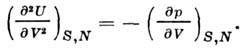
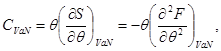
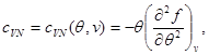
Heat capacity at DC volume is
![]()
However, this is not the only possible choice of independent variables that determine the P. t. They can be chosen by four decomp. ways, when one thermal and two mechanical are independent. values: S, V, N; S, p, N; T, V, N; T, p, N. In order to replace one of the independent variables by its conjugate in the total differential of type (1), we must perform Legendre transformation, i.e., subtract the product of two conjugate variables.
That. enthalpy can be obtained H(S, p, N) (Gibbs thermal function, heat content, isochoric - isothermal potential with independent variables S, p, N):
whence it follows that
Knowledge H allows you to find the heat capacity at DC. pressure
Free energy
F(T,V,N)(Helmholtz energy, heat content, isobaric-isothermal potential in variables T, V, N) can be obtained using the Legendre transform of the variables S, V, N to T, V, N:
where
Second derivatives F according to V p G give the heat capacity at DC. isothermal volume. coefficient pressure
and isochoric coefficient. pressure
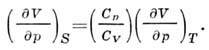
The last relation is based on the independence of the second mixed derivative of the P. t. from the order of differentiation. The same method can be used to find the difference between and :
and the ratio between adiabatic. and isothermal coefficient compression:
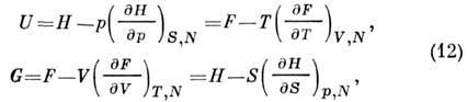
Gibbs energy (isobaric - isothermal potential in variables T, p, N) is related by the Legendre transformation to P. t. U, H, F:
where
Proportionality G number of particles makes it very convenient for applications, especially in theory phase transitions. Second derivatives G give heat capacity at post. pressure
![]()
and isothermal coefficient compression
From equations (3), (5), (6), (8) it follows that P. t. U, H, F, G connected :
to-rye used to build section. P. t. according to the ex-perim. thermal data. and calorie. ur-niyah state. The boundary conditions necessary for this are given by the passage to the limit to an ideal gas and Nernst theorem, which establishes that S=0 within the limit T Oh and so U=F and G - H.
For non-closed systems, for which N is not fixed, it is convenient to choose P. t. in variables T, V, which has not received a special name and is usually denoted ![]()
Its total differential
All P. t. are associated with various Gibbs distributions. P. t.
associated with the grand canon. Gibbs distribution by the relation
where - statistical integral over phase variables and the sum over N in the case of the classic mechanics or partition function on quantum states. P. t. F(T, V, N) is associated with the canonical Gibbs Ensemble:
where is a statistic. integral in classical case and statistical amount in quantum. P. t. H associated with isobaric-isothermal. the Gibbs Ensemble, which was proposed by S. A. Boguslavsky (1922). P. t. / 7 is associated with microcanonical. Gibbs distribution via entropy:
where W(U, V, N) - statistic. weight, to-ry is a normalization factor for microcanonical. Gibbs distribution. The total entropy differential is
which is equivalent to equation (1).
Statistical integrals or statistics. sums can in principle be calculated on the basis of the f-tion of Hamilton in the classical. case or the Hamiltonian operator in the quantum case for a system of a large number of interacting particles, and so on. calculate P. t. by statistical methods. mechanics.
In addition to the listed P. t., others are also used, for example. Massieux functions - F(T, V, N)IT, the Planck functions - ![]() In the general case, when a system with a given entropy is described by a thermodynamic parameters and their associated thermodynamic parameters. forces
In the general case, when a system with a given entropy is described by a thermodynamic parameters and their associated thermodynamic parameters. forces ![]()

and similarly for systems with fixed energy.
For polarizable media, P. t. depend on the electric vectors. and magn. induction D
and AT
. The method of P. t. allows you to find the tensors of the electric. and magn. permeability. In the isotropic case, the dielectric permeability is determined from the equations

The use of the P. t. method is especially effective in the case when there are connections between the parameters, for example. to study the conditions of thermodynamic. equilibrium of a heterogeneous system consisting of contiguous phases and decomp. component. In this case, if it is possible to neglect the ext. forces and surface phenomena, cf. the energy of each phase is ![]() where is the number of particles of the component i in phase k. Therefore, for each of the phases
where is the number of particles of the component i in phase k. Therefore, for each of the phases
(- chemical potential of component i in the phase k). P. t. U is minimal provided that the total number of particles of each component, the total entropy and volume of each phase remain constant.
Method P. t. allows you to explore the stability of thermodynamic. equilibrium of the system with respect to small variations of its thermodynamic. parameters. Equilibrium is characterized by max. the value of entropy or the minimum of its P. t. (internal energy, enthalpy, free energy, Gibbs energy), corresponding to independent thermodynamic experimental conditions. variables.
So, with independent S, V, N for balance, it is necessary that there be a minimum int. energy, i.e., with small variations in variables and with constancy S, V, N. Hence, as a necessary condition for equilibrium, the constancy of pressure and temperature of all phases and the equality of chemical. potentials of coexisting phases. However, for thermodynamic sustainability is not enough. From the condition of minimality of P. t. follows the positivity of the second variation: > 0. This leads to the conditions of thermodynamic. sustainability, eg. to a decrease in pressure with increasing volume and positive heat capacity at DC. volume. The P. t. method allows you to establish for multi-phase and multi-component systems Gibbs phase rule, according to which the number of phases coexisting in equilibrium does not exceed the number of independent components by more than two. This rule follows from the fact that the number of independent parameters cannot exceed the number of equations for their determination at phase equilibrium.
To build a thermodynamic theories, which would take into account surface phenomena, in the variations of P. t., one should take into account the terms proportional to the variations in the surface of the contacting phases. These terms are proportional surface tension s, which makes sense variats. derivative of any of the P. t. with respect to the surface.
The P. method is also applicable to continuous spatially inhomogeneous media. In this case, P. t. are functionals of thermodynamic. variables, and thermodynamic. equalities take the form of equations in functional derivatives.
Lit.: Vaals I.D. you der, Konstamm F., Thermostatics course, part 1. General thermostatic, trans. from German., M., 1936; Munster A., Chemical thermodynamics, trans. from German., M., 1971; Gibbs J. B., Thermodynamics. Statistical mechanics, trans. from English, M., 1982; Novikov I.I., Thermodynamics, M., 1984. D. N. Zubarev.
All calculations in thermodynamics are based on the use of state functions called thermodynamic potentials. Each set of independent parameters has its own thermodynamic potential. Changes in potentials that occur during any processes determine either the work done by the systole or the heat received by the system.
When considering thermodynamic potentials, we will use relation (103.22), presenting it in the form
The equal sign refers to reversible processes, the inequality sign - to non-reversible processes.
Thermodynamic potentials are state functions. Therefore, the increment of any of the potentials is equal to the total differential of the function by which it is expressed. The total differential of the function of variables and y is determined by the expression
![]()
Therefore, if in the course of transformations we obtain an expression of the form for the increment of a certain value
it can be argued that this quantity is a function of the parameters , and the functions are partial derivatives of the function
Internal energy. We are already familiar with one of the thermodynamic potentials. This is the internal energy of the system. The first law expression for a reversible process can be represented as
![]() (109.4)
(109.4)
Comparison with (109.2) shows that the variables S and V act as the so-called natural variables for the potential V. It follows from (109.3) that
![]()
It follows from the relation that in the case - when the body does not exchange heat with external environment, the work done by him is equal to
![]()
or in integral form:
Thus, in the absence of heat exchange with the external environment, the work is equal to the decrease in the internal energy of the body.
At, constant volume
Therefore, - the heat capacity at constant volume is equal to
![]() (109.8)
(109.8)
Free energy. According to (109.4), the work produced by heat with reversible isothermal process, can be represented as
State function
![]() (109.10)
(109.10)
called the free energy of the body.
In accordance with the formulas "(109.9) and (109.10) in a reversible isothermal process, the work is equal to the decrease in the free energy of the body:
![]()
Comparison with formula (109.6) shows that in isothermal processes free energy plays the same role as internal energy in adiabatic processes.
Note that formula (109.6) is valid for both reversible and irreversible processes. Formula (109.12) is valid only for reversible processes. With irreversible processes (see). Substituting this inequality into the relation, it is easy to obtain that for irreversible isothermal processes
Therefore, the loss of free energy determines the upper limit of the amount of work that the system can do in an isothermal process.
Let us take the differential of the function (109.10). Taking into account (109.4) we get:
From a comparison with (109.2) we conclude that the natural variables for the free energy are T and V. In accordance with (109.3)
Let's replace: in (109.1) dQ through and divide the resulting relation by ( - time). As a result, we get that
![]()
If the temperature and volume remain constant, then relation (109.16) can be converted to the form
It follows from this formula that an irreversible process occurring at constant temperature and volume is accompanied by a decrease in the free energy of the body. When equilibrium is reached, F stops changing with time. In this way; at constant T and V, the equilibrium state is the state for which the free energy is minimal.
Enthalpy. If the process “occurs at constant pressure, then the amount of heat received by the body can be represented as follows:
State function
![]()
called the enthalpy or heat function.
From (109.18) and (109.19) it follows that the amount of heat received by the body during the isobatic process is equal to
or in integral form
![]()
Therefore, in the case when the pressure remains constant, the amount of heat received by the body is equal to the increment of enthalpy. Differentiating the expression (109.19) with regard to (109.4) gives
From here we conclude. enthalpy is the thermodynamic potential in variables. Its partial derivatives are
![]()
If the temperature and pressure remain constant, relation (109.16) can be written as:
It follows from this formula that an irreversible process occurring at constant temperature and pressure is accompanied by a decrease in the thermodynamic Gibbs potential. When equilibrium is reached, G ceases to change with time. Thus, at constant T and the equilibrium state is the state for which the thermodynamic Gibbs potential is minimal (cf. (109.17)).
In table. 109.1 shows the basic properties of thermodynamic potentials.
Table 109.1

Lecture on the topic: “Thermodynamic potentials”
1. The group of potentials “E F G H” having the dimension of energy.
2. Dependence of thermodynamic potentials on the number of particles. Entropy as a thermodynamic potential.
3. Thermodynamic potentials of multicomponent systems.
4. Practical implementation of the method of thermodynamic potentials (on the example of the problem of chemical equilibrium).
One of the main methods of modern thermodynamics is the method of thermodynamic potentials. This method arose largely due to the use of potentials in classical mechanics, where its change was associated with the work performed, and the potential itself is an energy characteristic of a thermodynamic system. Historically, the initially introduced thermodynamic potentials also had the dimension of energy, which determined their name.
The mentioned group includes the following systems:
Internal energy;
Free energy or Helmholtz potential;
Gibbs thermodynamic potential;
Enthalpy.
The potentiality of internal energy was shown in the previous topic. It implies the potentiality of the remaining quantities.
The differentials of thermodynamic potentials take the form:
From relations (3.1) it can be seen that the corresponding thermodynamic potentials characterize the same thermodynamic system with different methods .... descriptions (methods of setting the state of a thermodynamic system). So, for adiabatically isolated system, described in variables, it is convenient to use internal energy as a thermodynamic potential. Then the parameters of the system, thermodynamically conjugated to the potentials, are determined from the relations:
If a "system in a thermostat" given by variables is used as a description method, it is most convenient to use free energy as a potential. Accordingly, for the system parameters we obtain:
Next, we will choose the “system under the piston” model as a way of describing it. In these cases, the state functions form a set (), and the Gibbs potential G is used as the thermodynamic potential. Then the system parameters are determined from the expressions:
And in the case of an “adiabatic system over a piston”, given by functions state, the role of the thermodynamic potential is played by the enthalpy H. Then the system parameters take the form:
Since relations (3.1) define complete differentials thermodynamic potentials, we can equate their second derivatives.
For example, given that
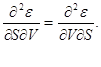
we get
Similarly, for the remaining parameters of the system related to the thermodynamic potential, we write:
Similar identities can also be written for other sets of parameters of the thermodynamic state of the system based on the potentiality of the corresponding thermodynamic functions.
So, for a “system in a thermostat” with a potential, we have:
For the system “above the piston” with the Gibbs potential, the equalities will be valid:
And, finally, for a system with an adiabatic piston with potential H, we get:
Equalities of the form (3.6) - (3.9) are called thermodynamic identities and in a number of cases turn out to be convenient for practical calculations.
The use of thermodynamic potentials makes it quite easy to determine the operation of the system and the thermal effect.
Thus, relations (3.1) imply:
From the first part of the equality follows the well-known provision that the work of a thermally insulated system () is carried out due to the decrease in its internal energy. The second equality means that the free energy is that part of the internal energy, which in the isothermal process is completely transformed into work (respectively, the “remaining” part of the internal energy is sometimes called bound energy).
The amount of heat can be represented as:
From the last equality it is clear why enthalpy is also called heat content. When burning and others chemical reactions occurring at constant pressure (), the amount of heat released is equal to the change in enthalpy.
Expression (3.11), taking into account the second law of thermodynamics (2.7), allows us to determine the heat capacity:

All thermodynamic potentials of the energy type have the property of additivity. Therefore, we can write:
It is easy to see that the Gibbs potential contains only one additive parameter, i.e. Gibbs specific potential does not depend on. Then from (3.4) it follows:
That is, the chemical potential is the specific Gibbs potential, and the equality takes place
The thermodynamic potentials (3.1) are interconnected by direct relations, which make it possible to make the transition from one potential to another. For example, let's express all thermodynamic potentials in terms of internal energy.
In doing so, we obtained all thermodynamic potentials as functions of (). In order to express them in other variables, use the procedure re….
Let pressure be given in variables ():
Let us write the last expression as an equation of state, i.e. find the form
It is easy to see that if the state is given in variables (), then the thermodynamic potential is the internal energy. By virtue of (3.2), we find
Considering (3.18) as an equation for S, we find its solution:
Substituting (3.19) into (3.17) we get
That is, from variables () we moved to variables ().
The second group of thermodynamic potentials arises if, in addition to those considered above, the chemical potential is included as thermodynamic variables. The potentials of the second group also have the dimension of energy and can be related to the potentials of the first group by the relations:
Accordingly, the potential differentials (3.21) have the form:
As well as for thermodynamic potentials of the first group, for potentials (3.21) one can construct thermodynamic identities, find expressions for the parameters of a thermodynamic system, and so on.
Let us consider the characteristic relations for the “omega potential”, which expresses the quasi-free energy and is used in practice most often among the other potentials of the group (3.22).
The potential is given in variables () describing the thermodynamic system with imaginary walls. The system parameters in this case are determined from the relations:
The thermodynamic identities following from potentiality have the form:
Quite interesting are the additive properties of the thermodynamic potentials of the second group. Since in this case the number of particles is not among the parameters of the system, the volume is used as an additive parameter. Then for the potential we get:
Here - specific potential per 1. Taking into account (3.23), we obtain:
Accordingly, (3.26)
The validity of (3.26) can also be proved on the basis of (3.15):
The potential can also be used to convert thermodynamic functions written in form to form. For this, relation (3.23) for N:
permitted regarding:
Not only the energy characteristics of the system, but also any other quantities included in relation (3.1) can act as thermodynamic potentials. As an important example, consider entropy as a thermodynamic potential. The initial differential relation for entropy follows from the generalized notation of the I and II principles of thermodynamics:
Thus, entropy is the thermodynamic potential for a system given by parameters. Other system parameters look like:
By resolving the first of relations (3.28), the passage from variables to variables is relatively possible.
The additive properties of entropy lead to the known relations:
Let us proceed to the determination of thermodynamic potentials on the basis of given macroscopic states of a thermodynamic system. To simplify calculations, we assume the absence of external fields (). This does not reduce the generality of the results, since additional systems simply appear in the resulting expressions for .
As an example, let us find expressions for free energy, using the equation of state, the caloric equation of state, and the behavior of the system at as initial ones. Taking into account (3.3) and (3.12), we find:
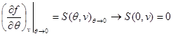
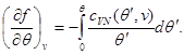
Let us integrate the second equation of system (3.30) taking into account the boundary condition at:

Then system (3.30) takes the form:
The solution of system (3.31) makes it possible to find the specific free energy in the form
The origin of the specific free energy can also be found from the conditions at:
Then (3.32) takes the form:
and the expression for the entire free energy of the system, up to an additive constant, takes the form:
Then the reaction of the system to the inclusion of an external field is given by an additional equation of state, which, depending on the set of state variables, has the form:
Then the change in the corresponding thermodynamic potential associated with the inclusion of zero from zero to is determined from the expressions:
Thus, setting the thermodynamic potential in the macroscopic theory is possible only on the basis of using given equations thermodynamic states, which, in turn, are themselves obtained on the basis of setting thermodynamic potentials. Break this " vicious circle” is possible only on the basis of microscopic theory, in which the state of the system is set on the basis of distribution functions, taking into account statistical features.
Let us generalize the obtained results to the case of multicomponent systems. This generalization is carried out by replacing the parameter with a set. Let's take a look at specific examples.
Let's assume that thermodynamic state system is given by parameters, i.e. we consider a system in a thermostat, consisting of several components, the number of particles in which is equal to The free energy, which in this description is the thermodynamic potential, has the form:
The additive parameter in (3.37) is not the number of particles, but the volume of the system V. Then the density of the system is denoted by . The function is a non-additive function of non-additive arguments. This is quite convenient, because when the system is divided into parts, the function does not change for each part.
Then, for the parameters of the thermodynamic system, we can write:
Considering that we have
For the chemical potential of an individual component, we write:
There are other ways to take into account the additive properties of free energy. Let us introduce the relative densities of the number of particles of each of the components:

independent of the volume of the system V. Here - total number particles in the system. Then
The expression for the chemical potential in this case takes a more complex form:
Calculate the derivatives of and and substitute them into the last expression:
The expression for pressure, on the contrary, will be simplified:
Similar relations can also be obtained for the Gibbs potential. So, if the volume is given as an additive parameter, then, taking into account (3.37) and (3.38), we write:
the same expression can be obtained from (3.yu), which in the case of many particles takes the form:
Substituting expression (3.39) into (3.45), we find:
which completely coincides with (3.44).
In order to go to the traditional Gibbs potential recording (through state variables ()) it is necessary to solve the equation (3.38):
Regarding the volume V and substitute the result in (3.44) or (3.45):
If the total number of particles in the system N is given as an additive parameter, then the Gibbs potential, taking into account (3.42), takes the following form:
Knowing the type of specific values: , we get:
In the last expression, summation over j replace by summation over i. Then the second and third terms add up to zero. Then for the Gibbs potential we finally obtain:
The same relation can be obtained in another way (from (3.41) and (3.43)):
Then for the chemical potential of each of the components we obtain:
In deriving (3.48), transformations similar to those used in deriving (3.42) were performed using imaginary walls. The system state parameters form a set ().
The role of the thermodynamic potential is played by the potential, which takes the form:
As can be seen from (3.49), the only additive parameter in this case is the volume of the system V.
Let us determine some thermodynamic parameters of such a system. The number of particles in this case is determined from the relation:
For free energy F and the Gibbs potential G can be written:
Thus, the relations for thermodynamic potentials and parameters in the case of multicomponent systems are modified only due to the need to take into account the number of particles (or chemical potentials) of each component. At the same time, the very idea of the method of thermodynamic potentials and calculations based on it remains unchanged.
As an example of using the method of thermodynamic potentials, consider the problem of chemical equilibrium. Let us find the conditions of chemical equilibrium in a mixture of three substances entering into a reaction. Additionally, we assume that the initial reaction products are rarefied gases (this allows us to ignore intermolecular mutual production), and the system maintains constant temperature and pressure, (such a process is the easiest to implement in practice, therefore the condition of constancy of pressure and temperature is created in industrial installations for a chemical reaction).
The equilibrium condition of a thermodynamic system, depending on the way it is described, is determined by the maximum entropy of the system or the minimum energy of the system (for more details, see Bazarov Thermodynamics). Then we can obtain the following equilibrium conditions for the system:
1. The state of equilibrium of an adiabatically isolated thermodynamic system, given by the parameters (), is characterized by a maximum of entropy:
The second expression in (3.53a) characterizes the stability of the equilibrium state.
2. The state of equilibrium of an isochoric-isothermal system, given by the parameters (), is characterized by a minimum of free energy. The equilibrium condition in this case takes the form:
3. The equilibrium of the isobaric-isothermal system, given by the parameters (), is characterized by the conditions:
4. For a system in a thermostat with a variable number of particles, defined by the parameters (), the equilibrium conditions are characterized by potential minima:
Let us turn to the use of chemical equilibrium in our case.
In the general case, the equation of a chemical reaction is written as:
Here are symbols chemical substances, - the so-called stoichiometric numbers. So for the reaction
Since pressure and temperature are chosen as parameters of the system, which are assumed to be constant. It is convenient to consider the Gibbs potential as a state of the thermodynamic potential G. Then the equilibrium condition for the system will consist in the requirement of the constancy of the potential G:
Since we are considering a three-component system, we set In addition, taking into account (3.54), we can write the balance equation for the number of particles ():
Introducing the chemical potentials for each of the components: and taking into account the assumptions made, we find:
Equation (3.57) was first obtained by Gibbs in 1876. and is the desired chemical equilibrium equation. It is easy to see, comparing (3.57) and (3.54), that the equation of chemical equilibrium is obtained from the equation of a chemical reaction by simply replacing the symbols of the reacting substances with their chemical potentials. This technique can also be used when writing the chemical equilibrium equation for an arbitrary reaction.
In the general case, the solution of equation (3.57), even for three components, is sufficiently loaded. This is due, firstly, to the fact that it is very difficult to obtain explicit expressions for the chemical potential even for a one-component system. Second, the relative concentrations and are not small quantities. That is, it is impossible to perform series expansion on them. This further complicates the problem of solving the equation of chemical equilibrium.
Physically noted difficulties are explained by the need to take into account the restructuring electron shells atoms that react. This leads to certain difficulties in the microscopic description, which also affects the macroscopic approach.
Since we agreed to confine ourselves to the study of gas rarefaction, we can use the model ideal gas. We assume that all reacting components are ideal gases that fill the total volume and create pressure p. In this case, any interaction (except chemical reactions) between the components of the gas mixture can be neglected. This allows us to assume that the chemical potential i-th component depends only on the parameters of the same component.
Here - partial pressure i-th component, and:
Taking into account (3.58), the equilibrium condition for the three-component system (3.57) takes the form:
For further analysis, we use the equation of state of an ideal gas, which we write in the form:
Here, as before, we denote the thermodynamic temperature. Then the record known from the school takes the form: , which is written in (3.60).
Then for each component of the mixture we get:
Let us determine the form of the expression for the chemical potential of an ideal gas. As follows from (2.22), the chemical potential has the form:
Taking into account equation (3.60), which can be written in the form, the problem of determining the chemical potential is reduced to determining the specific entropy and specific internal energy.
The system of equations for the specific entropy follows from the thermodynamic identities (3.8) and the heat capacity expression (3.12):
Taking into account the equation of state (3.60) and passing to the specific characteristics, we have:
Solution (3.63) has the form:
The system of equations for the specific internal energy of an ideal gas follows from (2.23):
The solution to this system can be written as:
Substituting (3.64) - (3.65) into (3.66) and taking into account the equation of state of an ideal gas, we obtain:
For a mixture of ideal gases, expression (3.66) takes the form:
Substituting (3.67) into (3.59), we get:
Performing transformations, we write:

Performing potentiation in the last expression, we have:
Relation (3.68) is called the law of mass action. The value is a function of temperature only and is called the component of a chemical reaction.
Thus, the chemical equilibrium and the direction of a chemical reaction is determined by the magnitude of pressure and temperature.
Thermodynamic potentials, Schuka, p.36
Thermodynamic potentials, Schuka, p.36
For isolated systems, this relation is equivalent to the classical formulation that entropy can never decrease. This conclusion was made by the Nobel laureate I. R. Prigozhy, analyzing open systems. He also advanced the principle that disequilibrium can serve as a source of order.
Third start thermodynamics describes the state of a system near absolute zero. In accordance with the third law of thermodynamics, it sets the entropy reference point and fixes it for any system. At T 0 vanish the coefficient of thermal expansion, the heat capacity of any process. This allows us to conclude that when absolute zero temperature, any change in state occurs without a change in entropy. This statement is called the theorem of the Nobel laureate V. G. Nernst, or the third law of thermodynamics.
The third law of thermodynamics says :
absolute zero is fundamentally unattainable because at T = 0 and S = 0.
If there were a body with a temperature equal to zero, then it would be possible to build a perpetual motion machine of the second kind, which contradicts the second law of thermodynamics.
Modification of the third law of thermodynamics to calculate the chemical equilibrium in the system formulated by the Nobel Prize winner M. Planck in this way.
Planck's postulate : at absolute zero temperature, the entropy takes on the value S 0 , independent of pressure, state of aggregation, and other characteristics of the substance. This value can be set to zero, orS 0 = 0.
According to statistical theory, the entropy value is expressed as S = ln, where is the Boltzmann constant, – statistical weight, or thermodynamic probability of macrostates. It is also called -potential. Under the statistical weight we mean the number of microstates, with the help of which a given macrostate is realized. The entropy of an ideal crystal at T = 0 K, subject to = 1, or in the case where the macrostate can be realized by a single microstate, is equal to zero. In all other cases, the value of entropy at absolute zero must be greater than zero.
3.3. Thermodynamic potentials
Thermodynamic potentials are functions of certain sets of thermodynamic parameters, allowing you to find all the thermodynamic characteristics of the system as a function of these same parameters.
Thermodynamic potentials completely determine the thermodynamic state of the system, and any system parameters can be calculated by differentiation and integration.
The main thermodynamic potentials include the following functions .
1. Internal energy U, which is a function of independent variables:
entropy S,
volume V,
number of particles N,
generalized coordinates x i
or U = U(S, V, N, x i).
2. Helmholtz free energy F is a function of temperature T, volume V, number of particles N, generalized coordinate x i so F = F(T, V, N, x t).
3. Gibbs thermodynamic potential G = G(T, p, N, x i).
4. Enthalpy H =H(S, P, N, x i).
5. Thermodynamic potential , for which the independent variables are temperature T, volume V, chemical potential x, = (T, V, N, x i).
There are classical relationships between thermodynamic potentials:
U = F + TS = H – PV,
F = U – TS = H – TS – PV,
H = U + PV = F + TS + PV,
G = U – TS + PV = F + PV = H – TS,
= U – TS – V = F – N = H – TS – N, (3.12)
U = G + TS – PV = + TS + N,
F = G – PV = + N,
H = G + TS = + TS + N,
G = + PV + N,
= G – PV – N.
The existence of thermodynamic potentials are a consequence of the first and second laws of thermodynamics and show that the internal energy of the system U depends only on the state of the system. The internal energy of the system depends on the full set of macroscopic parameters, but does not depend on how this state is reached. We write the internal energy in differential form
dU = TdS– PdV– X i dx i + dN,
T = ( U/ S) V, N, x= const ,
P = –( U/ V) S, N, x= const ,
= ( U/ N) S, N, x= const .
Similarly, one can write
dF = – SdT–PdV – X t dx t + dN,
dH= TdS+VdP– X t dx t + dN,
dG= – SdT+VdP – X i dx i + dN,
d = – SdT–PdV – X t dx t – Ndn,
S = – ( F/ T) V ; P = –( F/ V) T ; T = ( U/ S) V ; V = ( U/ P) T ;
S = – ( G/ T) P ; V = ( G/ P) S ; T = ( H/ S;); P = – ( U/ V) S
S = – ( F/ T); N = – ( F/); = ( F/ N); X = – ( U/ x).
These equations hold for equilibrium processes. Let us pay attention to the thermodynamic isobaric-isothermal potential G, called Gibbs free energy,
G = U – TS + PV = H –TS, (3.13)
and isochoric-isothermal potential
F = U – TS, (3.14)
which is called the Helmholtz free energy.
In chemical reactions occurring at constant pressure and temperature,
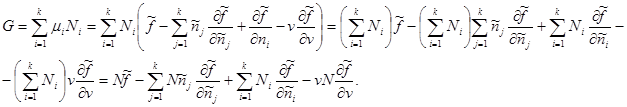
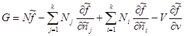
G = U – TS + PV = N, (3.15)
where is the chemical potential.
Under the chemical potential of some component of the system i we will understand the partial derivative of any of the thermodynamic potentials with respect to the amount of this component at constant values of the other thermodynamic variables.
Chemical potential can also be defined as a quantity that determines the change in the energy of the system when one particle of a substance is added, for example,
i = ( U/ N) S , V= cost , or G = i N i .
It follows from the last equation that = G/ N i , that is, is the Gibbs energy per particle. Chemical potential is measured in J/mol.
Omega potential is expressed through a large partition function Z how
= – T ln Z, (3.16)
Where [summation over N and k(N)]:
Z= exp[( N – E k (N))/T].


