The dependence of the potential difference on the distance. Potential difference, charge energy in an electric field. Potential

In the previous paragraph, we discussed the main characteristic electric field- his tension. As follows from the definition itself, this is a power characteristic, and therefore a vector. In some cases, scalar characteristics are more convenient, which, it turns out, can also be introduced for electrostatic field– potential difference and potential. In this case, we will rely on an important fundamental property of forces acting on a charge in an electrostatic field - their conservatism.

Recall that forces are called conservative, the work of which does not depend on the shape of the trajectory of the body. The work of such forces is determined only by the coordinates of the initial and final points of displacement. Based on our knowledge of the properties of its power characteristics of the electrostatic field created by an arbitrary system of charges, it would be possible to carry out a detailed proof of the equality of work when a charge moves between any two of its points. But we will somewhat shorten this procedure, recalling the theorem “on the conservativeness of central forces”, which we proved in the section on mechanics.

A stationary point charge is the source of the "field of central forces" - this directly follows from the formulation of the basic law of electrostatics - Coulomb's law. It follows from the principle of superposition of electric fields that the work done when a test charge moves in the field of any system resting charges is the algebraic sum of work in the field of each of the charges separately. This means that the field of such forces (“Coulomb forces” *)) is also a field of conservative forces. This is what needed to be proven.

Thus, the work of the forces of the electrostatic field **) on the movement of a point (trial) charge between two points characterizes this field. But it also depends on the magnitude of the test charge q 0 . This is evidenced by experience, but this is also understandable, based on our knowledge of the "Coulomb" forces. Because they are proportional to the charge q 0 at each point of the trajectory 1®2 (based on Coulomb's law), and the work is proportional to the force. To characterize the field and only the field, you can divide the work by the value of the test charge. What happens is the "potential difference". Here is a definition of this important concept:

(ODA .) Potential difference between electrostatic field points 1 and 2 is called attitude work fields by moving the test charge from the point 1exactly 2to the value of this charge :

. (3.1)

In the SI system, the unit of potential difference is called 1 volt (1 V = 1 J/C). If we learn how to somehow determine the potential difference j 1 –j 2 for the field of a system of charges at rest (theoretically or experimentally), this will allow us to find the work of the field by moving any pinpoint charge q in this field:

. (3.2)

So the potential difference is energy characteristic electric field, since it is directly related to the concept of work.

In mechanics, we introduced the concept of "potential energy" for conservative forces (now we say: "fields of conservative forces"). At the same time, we were guided by the following principle: “the work of the field forces is equal to the loss potential energy". We formalize this principle in an analytical notation:

Here U 1 and U 2 are the potential energy in the "initial" ("1") and "final" ("2") states of the system, respectively. In the case under discussion, the fields of the system of fixed charges are the energy point charge q in position "1" (with coordinates ( x 1 ,y 1 ,z 1 )) and position "2" (with coordinates ( x 2 ,y 2 ,z 2 )) electrostatic field. Those. the potential energy of the charge in this field is a scalar function of the coordinates of the field points U = U( x,y,z) (or ). Comparing (3.2) and (3.3), we see that it is convenient to assume that the potential difference is the difference in the values of another scalar function of the coordinates of the field points j(x,y,z). It is related to the function U( x,y,z) (potential energy) by a simple relation: U( x,y,z) = q× j(x,y,z). Or because

it is said to be "numerically equal to the potential energy of a unit positive charge" at a given point in the field. And this value is called j the "potential" of a given point of the electrostatic field.

The most important thing is how to find this function for the field of a particular system of charges? What is the procedure?

First of all, we have to agree on the normalization conditions *): we need to choose a point R 0 , in which the test charge potential will be assumed to be equal to zero . Most often, such a point is chosen "infinitely" remote, where the field is absent **). To do this, you need to find the "specific" work of the field - i.e. work related to the amount of test charge transferred (or, as it is often said, "by moving a unit positive" charge) from a given point in the field R(x,y,z) to the normalization point R 0 . In analytical form, this definition potential can be written as follows:

(Def. ) j P(x,y,z) = . (3.5)

Is it possible to express the values newly introduced by us - the potential difference and the potential through the power characteristic, which we have already learned how to calculate by given location charges in space? Yes, you certainly may. Let us write down a chain of equalities that are well understood to us:

Let's write the last equation again

. (3.6)

It gives a "recipe" for searching for a potential difference using a known function of tension. Similarly for the potential:

And finally for the potential of an arbitrary point of the field R with coordinates ( x,y,z):

. (3.7)

· Potential of the field of a point charge

Based on the procedure for calculating the potential, we obtain an expression for the case of a point charge field. This is very important for further calculations of the field potential of a system of charges arbitrarily located in space.

2. Choice of trajectory. Let an arbitrary point R(x,y,z) is at a distance r from the source charge. Since the result does not depend on the shape of the trajectory, for calculating the curvilinear integral of the form (3.7) we choose the simplest radially directed straight line from a given point of the field along the field line and “going to infinity”.

3. Calculation. In accordance with the definition of the potential, we calculate the "specific" work of the field created by a point charge q on the transfer of test charge along the chosen trajectory. The following chain of equalities, we hope, looks quite "transparent". However, we will still give a minimal comment to it. First of all, we note that due to our choice of a trajectory in the form of a ray directed radially from the charge, we can denote E l and dl(arbitrary curve " L") change to Er and dr(polar axis " r"). Moreover, since the vector is directed radially, for any small displacement along the trajectory, the projection of the stress vector is simply equal to the modulus of this vector E(r). As a result, we can also take an important step in our calculation - to make the transition from the curvilinear integral to the usual definite one:

.*)

Now, after substituting the expression for the modulus of the field strength of a point charge (3.5), we are left with just a mathematical “routine”:

Let us write the result again, supplementing it with the possible presence of a gaseous or liquid homogeneous dielectric medium with a permittivity e, which fills the entire space surrounding the point charge:

. (3.8)

The field potential of a point charge, as we see, decreases with distance according to the law 1/ r.

· Equipotential surfaces

When discussing power characteristics electrostatic field, we were convinced of the fruitfulness of the concept lines of force(tension lines). For the energy characteristic of the field - potential - it is also useful to introduce an additional illustrative characteristic - a system of "equipotential surfaces". From the name itself it is clear (“equi” means “equal”) that these are surfaces of constant potential, which characterize the ability of field forces to do work when moving a charge. Along such surfaces, obviously, no work is done at all. It is maximum in the directions along which the density (density) of equipotential surfaces is maximum. In these places, the field strength is also maximum. It is easy to figure out what is the mutual orientation of the lines of force and equipotential surfaces at their intersections: they are mutually perpendicular. After all, for any small displacement along the equipotential surface elementary work is equal to zero, and this is possible only if the tangent component of the stress vector is equal to zero, i.e. it is directed strictly along the normal to the surface. Below we give a chain of corresponding to these words, we hope, fairly obvious equalities:

Together with Fig. 3. ... they prove, in fact, the already formulated statement: lines of force cross (or "coming to...") equipotential surfaces at right angles !

Let's give a picture of equipotential surfaces (and lines of force too) for some of the simplest cases of an electrostatic field that are already well known to us: a) field of a point charge; b) the field of two identical in absolute value opposite point charges; in) the field between two oppositely charged plane-parallel large (compared to the distance between them) plates - see fig. 3.1.

Let us now turn to a spherical (point) charge. It is shown above that the strength of the electric field created by a charge uniformly distributed over the sphere Q, does not depend on the radius of the sphere. Imagine that at some distance r from the center of the sphere is a test charge q. The field strength at the point where the charge is located,

The figure shows a graph of the dependence of the strength of the electrostatic interaction between point charges on the distance between them. To find the work of the electric field when moving the test charge q from a distance r up to a distance R, divide this interval by points r 1 , r 2 ,..., rP into equal sections. Average force acting on a charge q within the interval [ rr 1 ] is equal to

The work of this force in this area:

Similar expressions for work will be obtained for all other sections. So the full job is:

Identical terms with opposite signs are destroyed, and finally we get:

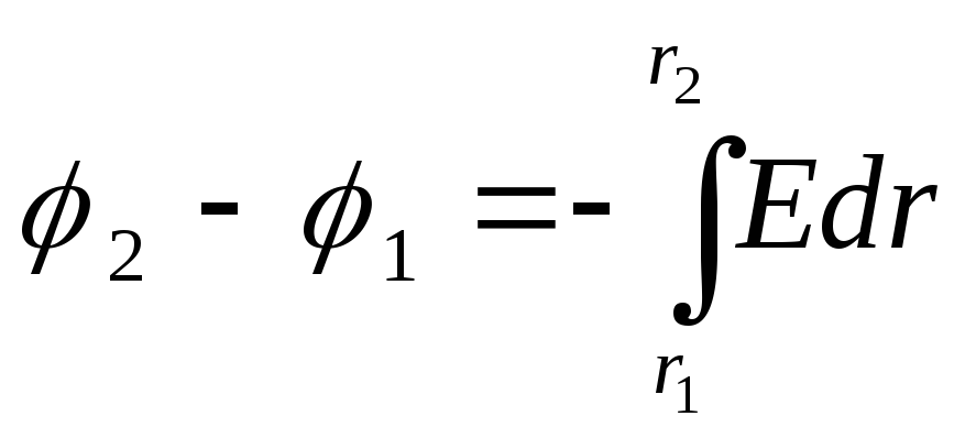
is the work of the field on the charge

– potential difference

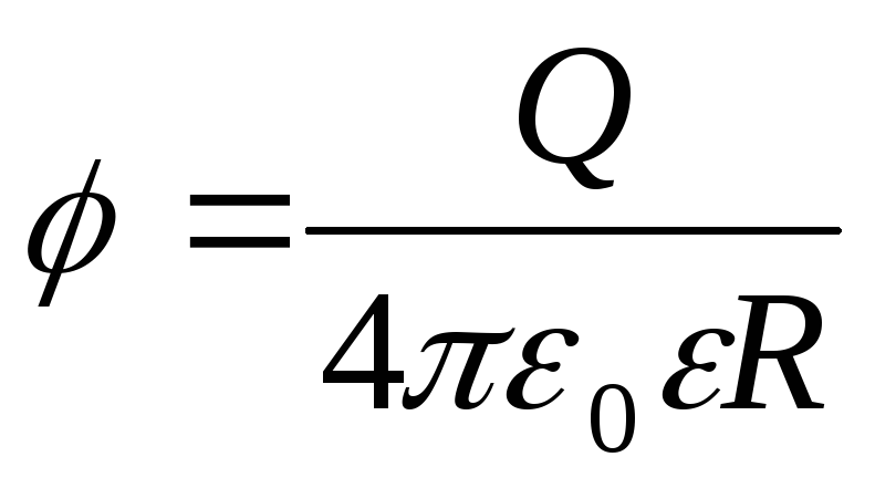
Now, in order to find the potential of the field point with respect to infinity, we direct R to infinity and finally we get:

So, the potential of the field of a point charge is inversely proportional to the distance to the charge.

24. Potential energy of a charge in the field of a system of charges. Superposition principle for potentials. Superposition principle for potentials

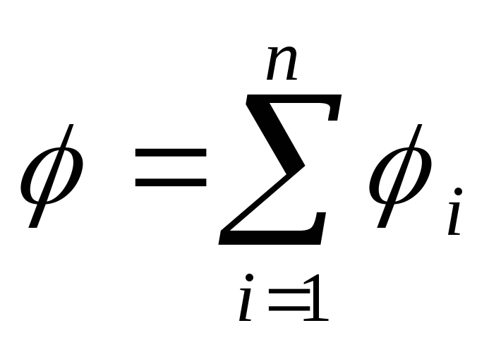
Any arbitrarily complex electrostatic field can be represented as a superposition of the fields of point charges. Each such field at the selected point has a certain potential. Since the potential is a scalar quantity, the resulting potential of the field of all point charges is the algebraic sum of the potentials 1, 2, 3, ... of the fields of individual charges: = 1 + 2 + 3 + ... This relation is a direct consequence of the principle of superposition of electric fields.

Potential energy of a charge in an electric field. Let's continue the comparison of the gravitational interaction of bodies and the electrostatic interaction of charges. body mass m in the Earth's gravitational field has potential energy. The work of gravity is equal to the change in potential energy, taken with the opposite sign:

A=-(W p2 - W p1) = mgh.

(Here and below we will denote the energy by the letter W.) Just like a body of mass m in the field of gravity has a potential energy proportional to the mass of the body, an electric charge in an electrostatic field has a potential energy W p , proportional to the charge q. The work of the forces of the electrostatic field BUT is equal to the change in the potential energy of the charge in the electric field, taken with the opposite sign:

A=-(W p2 - W p1) . (40.1)

25. Potential difference. Equipotential surfaces

Equipotential surface- a surface, each point of which has the same potential.

As follows from the connection between work and potentials:

when charge is transferred along equipotential surfaces, the electric field does no work, since .

Work with a non-zero force is zero only if the force vector is perpendicular to the displacement vector. It follows from this that the lines of tension are perpendicular to the equipotential surfaces. Examples of equipotential surfaces are spheres for the field of a point charge and parallel planes for homogeneous fields (Fig. 3).

Potential difference (voltage) between two points is equal to the ratio of the field work when moving the charge from the starting point to the final point to the module of this charge: U\u003d φ 1 - φ 2 \u003d -Δφ \u003d A / q, A \u003d - (W p2 - W p1) \u003d -q (φ 2 - φ 1) \u003d -qΔφ

The potential difference is measured in volts (V = J / C) The relationship between the strength of the electrostatic field and the potential difference: E x = Δφ / Δ x The strength of the electrostatic field is directed in the direction of decreasing potential. Measured in volts divided by meters (V/m)

§ 15. POTENTIAL. ENERGY OF THE SYSTEM OF ELECTRIC CHARGES. WORK ON MOVING THE CHARGE IN THE FIELD

Basic Formulas

 The potential of an electric field is a value equal to the ratio of the potential energy of a point positive charge placed in given point fields, to this charge;

=P/ Q,

or the potential of the electric field is a quantity equal to the ratio of the work of the field forces to move a point positive charge from a given point of the field to infinity to this charge:

=A/ Q.

The potential of the electric field at infinity is conditionally taken equal to zero.

Note that when a charge moves in an electric field, the work A v.s external forces is equal in absolute value to the work A s.p. field strength and is opposite to it in sign:

A v.s = – A s.p. .

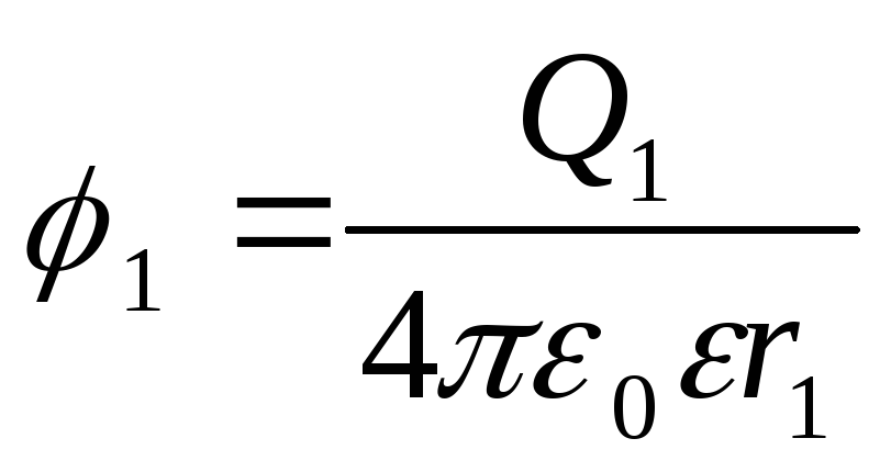
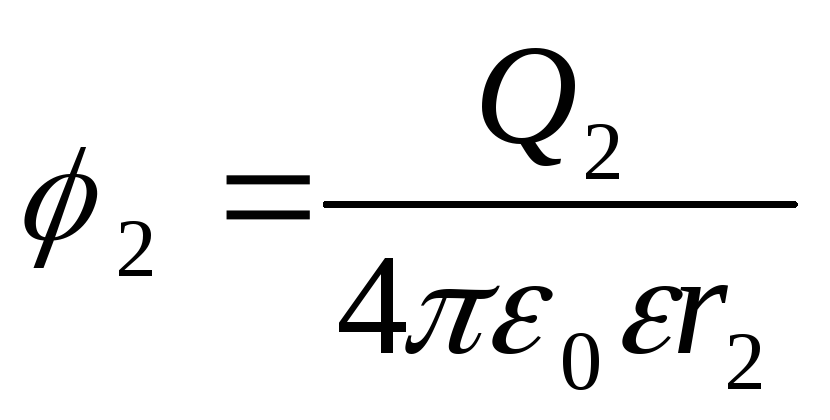
 Electric field potential created by a point charge Q on distance r from the charge

 The potential of the electric field created by the metal, carrying a charge Q sphere with radius R, at a distance from the center of the sphere:

inside the sphere ( r<R)

;

on the surface of a sphere ( r=R)

;

out of scope (r> R)

.

In all the formulas given for the potential of a charged sphere,  is the permittivity of a homogeneous infinite dielectric surrounding the sphere.

 The potential of the electric field created by the system P point charges, at a given point, in accordance with the principle of superposition of electric fields, is equal to the algebraic sum of potentials  1 , 2 , ... , n, created by individual point charges Q 1 ,Q 2 , ...,Q n :

 Energy W interactions of a system of point charges Q 1 ,Q 2 , ...,Q n is determined by the work that this system of charges can do when they are removed relative to each other to infinity, and is expressed by the formula

where  i- the potential of the field created by all P- 1 charges (excluding the 1st) at the point where the charge is located Q i .

 The potential is related to the strength of the electric field by the relation

E= -grad.

In the case of an electric field with spherical symmetry, this relationship is expressed by the formula

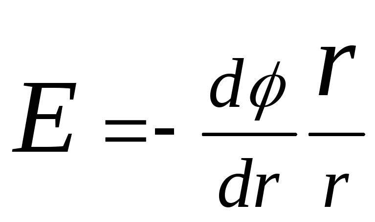or in scalar form

and in case uniform field, i.e., a field whose intensity at each point is the same both in absolute value and in direction,

E=( 1 – 2 ,)/d,

where  1 and 2 - potentials of points of two equipotential surfaces; d - the distance between these surfaces along the electrical field line.

 Work done by an electric field when moving a point charge Q from one point of the field with a potential  1 , into another with a potential  2 ,

A=Q( 1 - 2 ), or

,

where E l - tension vector projection E to the direction of movement; dl - movement.

In the case of a homogeneous field, the last formula takes the form

A= QElcos ,

where l- displacement;  - angle between vector directions E and displacement l.

Examples of problem solving

Example 1 positive charges Q 1 \u003d 3 μC and Q 2 \u003d 20 nC are in vacuum at a distance r 1 =l.5 m apart. Define a job A, which must be done in order to bring the charges closer to a distance r 2 =1 m.

Solution. Let us assume that the first charge Q 1 remains stationary and the other Q 2 under the action of external forces moves in the field created by the charge Q 1 approaching him from a distance r 1 =t,5 m up to r 2 =1 m .

Work BUT" external force to move the charge Q from one point of the field with potential  1 into another, whose potential 2 , equal in absolute value and opposite in sign to work BUT field forces for the movement of the charge between the same points:

A "= -A.

Work BUT field forces on charge displacement A=Q( 1 - 2 ). Then work BUT" external forces can be written as

A" = –Q( 1 - 2 )=Q( 2 - 1 ). (1)

The potentials of the start and end points of the path are expressed by the formulas

;

.

Substituting expressions  1 and 2 into formula (1) and taking into account that for this case the transferred charge Q=Q 2 , we get

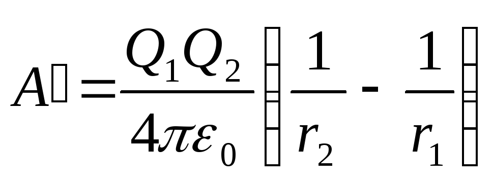. (2)

Considering that 1/(4 0 )=910 9 m/F, then after substituting the values of the quantities into formula (2) and calculating, we find

A"=180 µJ.

Example 2 Find a job BUT charge transfer fields Q=10 nC from point 1 exactly 2 (Fig. 15.1), located between two oppositely charged ones with a surface density  \u003d 0.4 μC / m 2 infinite parallel planes, distance l between them is 3 cm.

R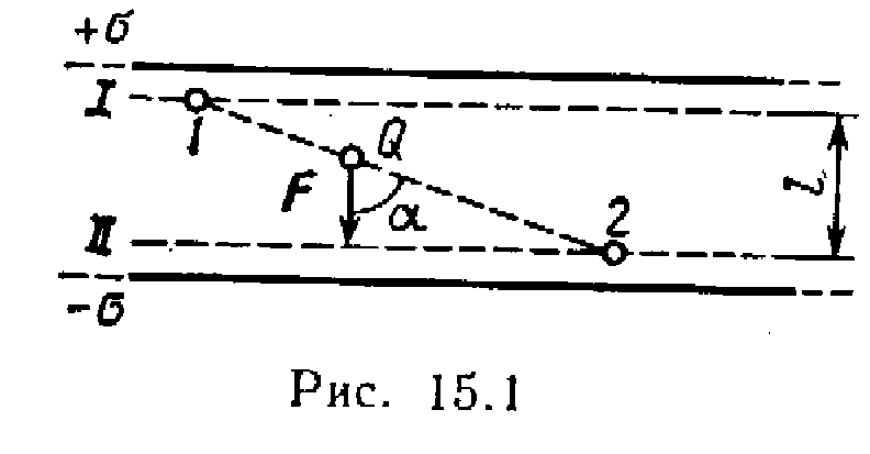

solution. There are two ways to solve the problem.

1st way. The work of the field forces to move the charge Q from the point 1 fields with potential 1 exactly 2 fields with potential 2 find by formula

A=Q( 1 - 2 ). (1)

To determine potentials at points 1 and 2 Let us draw equipotential surfaces I and II through these points. These surfaces will be planes, since the field between two uniformly charged infinite parallel planes is uniform. For such a field, the relation

 1 - 2 =El, (2)

where E - field strength; l - distance between equipotential surfaces.

Field strength between parallel infinite oppositely charged planes E=/ 0 . Substituting this expression E into formula (2) and then the expression 1 - 2 into formula (1), we obtain

A= Q( /  0 ) l.

2nd way. Since the field is uniform, the force acting on the charge Q, is constant as it moves. Therefore, the work of moving the charge from the point 1 exactly 2 can be calculated using the formula

A=F  r cos, (3)

where F - force acting on a charge r- charge transfer module Q from a point 1 exactly 2;  is the angle between the directions of displacement and force . But F= QE= Q( /  0 ). Substituting this expression F into equality (3), as well as noticing that  r cos= l, we get

A=Q(/ 0 )l. (4)

Thus, both solutions lead to the same result.

Substituting into expression (4) the value of quantities Q, , 0 and l, find

A\u003d 13.6 μJ.

Example 3 On a thin thread bent along an arc of a circle with a radius R, uniformly distributed charge with linear density=10 nC/m. Define tension E and potential  of the electric field created by such a p

distributed charge at a point O, coinciding with the center of curvature of the arc. Length l the thread is 1/3 of the circumference and is equal to 15 cm.

Solution. We choose the coordinate axes so that the origin of coordinates coincides with the center of curvature of the arc, and the axis at was symmetrically located relative to the ends of the arc (Fig. 15.2). Select an element of length d on the thread l. Charged Q=d l, located in the selected area, can be considered as a point.

Let us determine the strength of the electric field at the point O. To do this, we first find the tension d E field created by the charge d Q:

where r-radius-vector directed away from element d l to the point at which the tension is calculated. We express the vector d E through projection dE x c and dE y on the coordinate axis:

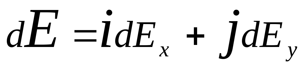where i and j- unit direction vectors (orths).

tension E find by integration:

Integration is carried out along the arc of length l. Due to symmetry, the integral equals zero. Then

, (1)

where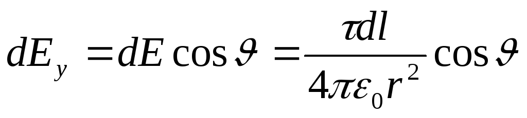

. Because r=R= const and d l=R d. then

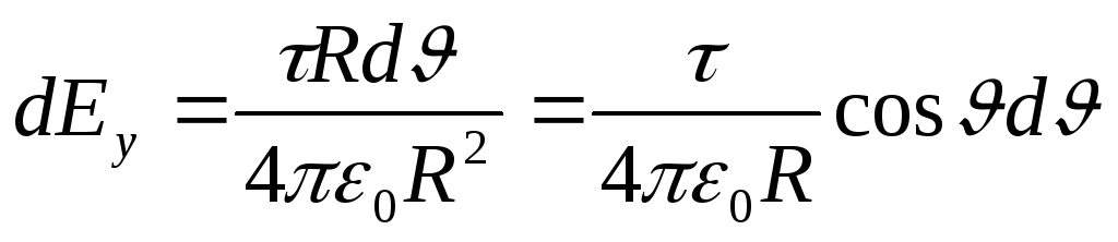
Substitute the found expression dE y in (1) and, taking into account the symmetrical location of the arc relative to the axis OU, we take the limits of integration from 0 to /3, and double the result;

Substituting these limits and expressing R through the length of the arc (3 l= 2 r), we get

This formula shows that the vector E coincides with the positive direction of the axis OU Substituting the value and l into the last formula and doing the calculations, we find

E\u003d 2.18 kV / m.

Let us determine the potential of the electric field at the point O. Let us first find the potential d created by the point charge d Q at the point O:

Let's replace r on the R and perform the integration:

.Because l=2  R/3, then

=/(6 0 ).

Having made calculations according to this formula, we obtain

Example4 . The electric field is created by a long cylinder with a radius R= 1cm , uniformly charged with linear density=20 nC/m. Determine the potential difference of two points of this field located at distances a 1 =0.5 cm and a 2 \u003d 2 cm from the surface of the cylinder, in its middle part.

Solution. To determine the potential difference, we use the relationship between the field strength and the change in potential E= -grad. For a field with axial symmetry, which is the field of a cylinder, this relation can be written as

E= -( d/d r) , or d= - E d r.

Integrating the last expression, we find the potential difference of two points separated by r 1 and r 2 from the axis of the cylinder;

. (1)

Since the cylinder is long and the points are taken near its middle part, the field strength can be expressed using the formula

. Substituting this expression E into equality (1), we obtain

(2)

Since the quantities r 2 and r 1 enter the formula as a ratio, then they can be expressed in any, but only the same units:

r 1 =R+a 1 = 1.5 cm; r 2 =R+a 2 =3cm .

Substituting the magnitude values , 0 ,r 1 and r 2 into formula (2) and calculating, we find

 1 - 2 =250 V.

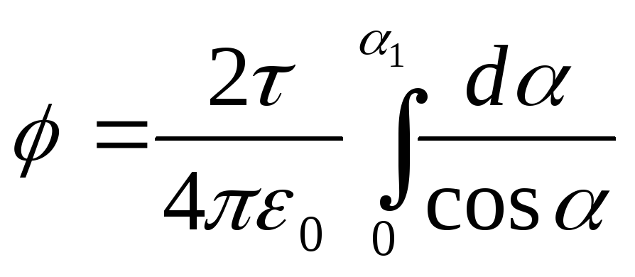
Example 5 The electric field is created by a thin rod carrying a charge =0.1 μC/m uniformly distributed along its length. Determine the potential  of the field at a point remote from the ends of the rod at a distance, equal to the length rod.

Solution. The charge on the rod cannot be considered as a point charge, therefore, directly apply the formula to calculate the potential

, (1)

valid only for point charges, it is impossible. But if we split the rod into elementary segments d l, then the charged l located on each of them can be considered as a point and then formula (1) will be valid. Applying this formula, we get

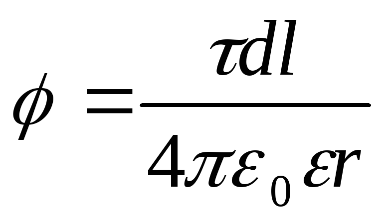, (2)

where r - the distance of the point at which the potential is determined to the rod element.

From fig. 15.3 that d l=(r d/cos). Substituting this expression d l into formula (2), we find

.

Integrating the resulting expression within the limits of  1 yes 2 , we obtain the potential created by the entire charge distributed on the rod: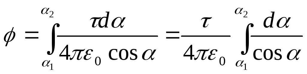

.

AT 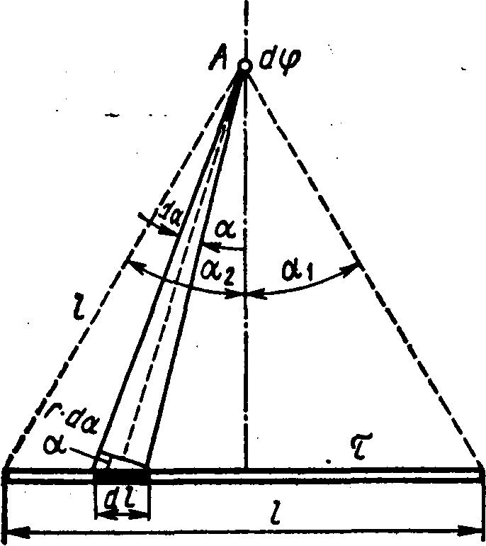point symmetry force BUT relative to the ends of the rod we have  2 = 1 and therefore

.

Consequently,

.Because

(see Table 2), then

.

Substituting the limits of integration, we obtain

Having made calculations according to this formula, we find

Example 6 An electron with a speed v=1.8310 6 m/s flew into a uniform electric field in the direction opposite to the field strength vector. What potential difference U an electron must pass in order to have energy E i\u003d 13.6 eV *? (Having such an energy, an electron can ionize it when it collides with a hydrogen atom. The energy of 13.6 eV is called the ionization energy of hydrogen.)

Solution. The electron must pass such a potential difference u, so that the energy acquired W combined with kinetic energy T, which the electron had before entering the field, amounted to an energy equal to the ionization energy E i , i.e. W+ T= E i . Expressing in this formula W= EU and T=(m v 2 /2), we get EU+(m v 2 /2)=E i. From here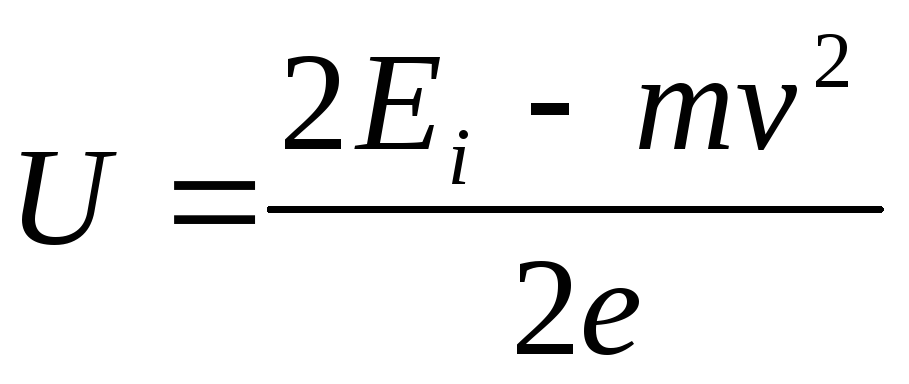

.

___________________

* Electron-volt (eV) - the energy acquired by a particle having a charge equal to the charge of an electron that has passed through a potential difference of 1 V. This non-systemic unit of energy is currently approved for use in physics.

Let's make calculations in SI units:

U=4.15 AT.

Example 7 Determine initial speed υ 0 approach of protons located at a sufficiently long distance from each other if the minimum distance r min , by which they can get close, is 10 -11 cm.

Solution: There are repulsive forces between the two protons, as a result of which the movement of the protons will be slow. Therefore, the problem can be solved as inertial system coordinates (associated with the center of mass of two protons), and in non-inertial (associated with one of the rapidly moving protons). In the second case, Newton's laws do not hold. The application of the d'Alembert principle is difficult due to the fact that the acceleration of the system will be variable. Therefore, it is convenient to consider the problem in an inertial frame of reference.

Let us place the origin of coordinates at the center of mass of two protons. Since we are dealing with identical particles, the center of mass will be at the point that bisects the segment connecting the particles. Relative to the center of mass, the particles will have at any time the same velocities modulo. When the particles are at a sufficiently large distance from each other, the speed υ 1 each particle is equal to half υ 0 , i.e. υ 1 =υ 0 /2.

To solve the problem, we apply the law of conservation of energy, according to which the total mechanical energy E isolated system is constant, i.e.

E=T+ P ,

where T- the sum of the kinetic energies of both protons relative to the center of mass; P is the potential energy of the system of charges.

We express the potential energy in the initial P 1 and final P 2 moments of motion.

At the initial moment, according to the condition of the problem, the protons were at a great distance, so the potential energy can be neglected (P 1 =0). Therefore, for the initial moment total energy will be equal to the kinetic energy T 1 protons, i.e.

E=T l . (1)

At the final moment, when the protons approach as close as possible, the speed and kinetic energy are equal to zero, and the total energy will be equal to the potential energy P 2, i.e.

E= P 2 . (2)

Equating the right parts of equalities (1) and (2), we obtain

T 1 \u003d P 2. (3)

The kinetic energy is equal to the sum of the kinetic energies of the protons:

(4)

Potential energy of a system of two charges Q 1 and Q 2 in vacuum is determined by the formula

, where r- distance between charges. Using this formula, we get

(5)

Taking into account equalities (4) and (5), formula (3) takes the form

where

After performing calculations according to the obtained formula, we find υ 0 =2,35 mm/s

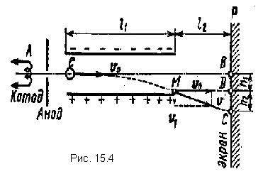Example 8 An electron without an initial velocity has passed the potential difference U 0 =10 kV and flew into the space between the plates of a flat capacitor charged to a potential difference U l \u003d 100 V, along the line AB, parallel to the plates (Fig. 15.4). Distance d between the plates is 2 cm. Length l 1 capacitor plates in the direction of electron flight is equal to 20cm. Determine distance Sun on the screen R, away from the condenser l 2 \u003d 1 m.

Solution. The motion of an electron inside the capacitor consists of two motions: 1) by inertia along the line AB at a constant speed υ 0 , acquired under the action of a potential difference U 0 , which the electron passed to the capacitor; 2) uniformly accelerated movement in the vertical direction to a positively charged plate under the action of a constant field force of the capacitor. After leaving the capacitor, the electron will move uniformly with a speed υ, which he had at the point M at the time of exit from the condenser.

From fig. 15.4 shows that the desired distance | | BC|=h 1 +h 2 , where from h 1 - the distance that the electron will move in the vertical direction while moving in the capacitor; h 2 - the distance between the point D on the screen, in which the electron would fall, moving at the exit from the capacitor in the direction of the initial velocity υ 0 , and the point C, where the electron actually hits.

Express separately h 1 and h 2 . Using the formula for the path length of uniformly accelerated motion, we find

. (1)

where a- acceleration received by the electron under the action of the capacitor field; t- the flight time of an electron inside a capacitor.

According to Newton's second law a=F/m, where F- the force with which the field acts on the electron; t- its mass. In its turn, F=eE=eU 1 /d, where e- electron charge; U 1 - potential difference between the capacitor plates; d- the distance between them. We find the flight time of an electron inside the capacitor from the formula for the path of uniform motion

, where

where l 1 is the length of the capacitor in the direction of electron flight. We find the expression for the speed from the condition of equality of the work done by the field when moving the electron and the kinetic energy acquired by it:

. From here

(2)

Substituting into formula (1) successively the values a,F, t and υ 0 2 from the corresponding expressions, we obtain

Cut length h 2 find from the similarity of triangles MDC and vector:

(3)

where υ 1 - electron speed in the vertical direction at a point M;l 2 - distance from the capacitor to the screen.

Speed υ 1 we find by the formula υ 1 =at, which, taking into account the expressions for a, F and t will take the form

Substituting the expression υ 1 into formula (3), we get

, or by replacing υ 0 2 by formula (3), we find

Finally for the required distance | BC| will have

|BC|=

Substituting the values of quantities U 1 ,U 0 ,d,l 1 and l 2 into the last expression and performing calculations, we get | BC|=5.5 cm.

Tasks

Potential energy and field potential of point charges

15.1. point charge Q\u003d 10 nC, being at a certain point in the field, has a potential energy P \u003d 10 μJ. Find the potential φ of this field point.

5.2. When moving charge Q=20 nC between two points of the field, work was done by external forces A=4µJ. Define a job A 1 field forces and the difference Δφ of the potentials of these points of the field.

15.3. The electric field is created by a point positive charge Q 1 \u003d 6 nC. positive charge Q 2 is transferred from the point BUT this field to a point AT(Fig. 15.5). What is the change in potential energy ΔP per unit of transferred charge, if r 1 =20 cm and r 2 \u003d 50 cm?

15.4. Electric field created by a point charge Q l \u003d 50 nC. Without using the concept of potential, calculate the work BUT in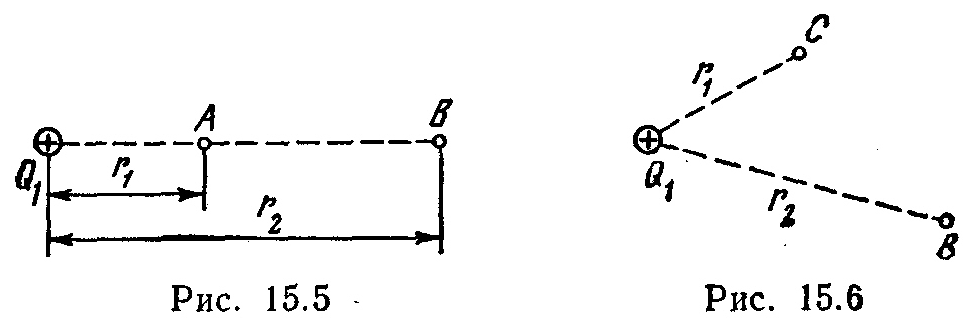

external forces to move a point charge Q 2 = -2 nC from point FROM exactly AT

(Fig. 15.6), if r 1 =10 cm, r 2 \u003d 20 cm. Also determine the change ΔP of the potential energy of the system of charges.

15.5. The field is created by a point charge Q=1 nC. Determine the potential φ of the field at a point remote from the charge at a distance r=20 cm.

15.6. Determine the potential φ of the electric field at a point remote from the charges Q 1 = -0.2 µC and Q 2 =0,5 μC, respectively, on r 1 =15 mass media r 2 \u003d 25 cm. Also determine the minimum and maximum distances between charges for which a solution is possible.

15.7. Charges Q 1 \u003d 1 μC and Q 2 = -1 μC are at a distance d\u003d 10 cm. Determine the tension E and potential φ of the field at a point remote at a distance r= 10 cm from the first charge and lying on a line passing through the first charge perpendicular to the direction from Q 1 to Q 2 .

15.8. Calculate the potential energy P of a system of two point charges Q 1 =100 nC and Q 2 =10 nC at a distance d=10 cm apart.

15.9. Find the potential energy P of a system of three point charges Q 1 \u003d 10 nC, Q 2 =20 nCl and Q 3 \u003d -30 nC, located at the vertices of an equilateral triangle with side length a=10 cm.

15.10. What is the potential energy P of a system of four identical point charges Q\u003d 10 nC, located at the vertices of a square with a side length a\u003d 10 cm? .

15.11. Determine the potential energy P of a system of four point charges located at the vertices of a square with side length a\u003d 10 cm. The charges are the same in modulus Q=10 nC, but two of them are negative. Consider two possible cases of the arrangement of charges.

15.12 . The field is created by two point charges + 2Q and -Q, at a distance d=12 cm apart. Determine the locus of points on the plane for which the potential is zero (write the equation for the line of zero potential).

5.13. The system consists of three charges - two of the same size Q 1 = |Q 2 |=1 μC and opposite in sign and charge Q=20 nC, located at point 1 in the middle between the other two charges of the system (Fig. 15.7). Determine the change in the potential energy ΔP of the system during charge transfer Q from point 1 to point 2. These points are removed from the negative charge Q 1 per distance a= 0,2 m.

Potential of the field of linearly distributed charges

15.14. Along a thin ring with a radius R= 10 cm uniformly distributed charge with a linear density τ= 10 nC/m. Determine the potential φ at a point lying on the axis of the ring, at a distance a= 5 cm from the center.

15.15. On a segment of a thin straight conductor, a charge is uniformly distributed with a linear density τ=10 nC/m. Calculate the potential φ created by this charge at a point located on the axis of the conductor and remote from the nearest end of the segment by a distance equal to the length of this segment.

Lecture 6. Electric field potential. Test No. 2

Potential is one of the most complex concepts of electrostatics. Students learn the definition of the potential of an electrostatic field, solve numerous problems, but they do not have a sense of potential, they have difficulty relating theory to reality. Therefore, the role of the educational experiment in the formation of the concept of potential is very high. We need such experiments that, on the one hand, would illustrate abstract theoretical ideas about the potential, and, on the other hand, show the complete validity of the experiment for introducing the concept of potential. It is rather harmful than useful to strive for special accuracy of quantitative results in these experiments.

6.1. Potentiality of the electrostatic field

Let us fix the conducting body on an insulating support and charge it. We hang a light conducting ball on a long insulated thread and give it a test charge, which is the same name as the body charge. The ball will bounce off the body and out of position 1 will move to position 2. Since the height of the ball in the gravitational field has increased by h, the potential energy of its interaction with the Earth has increased by mgh. This means that the electric field of the charged body has done some work on the test charge.

Let's repeat the experiment, but at the initial moment, let's not just let go of the test ball, but push it in an arbitrary direction, giving it some kinetic energy. At the same time, we find that moving from the position 1 along a complex trajectory, the ball will eventually stop in the position 2 . Informed to the ball at the initial moment kinetic energy, obviously, was spent on overcoming the forces of friction during the movement of the ball, and the electric field did the same work on the ball as in the first case. Indeed, if we remove the charged body, then the same push of the test ball leads to the fact that from the position 2 he returns to position 1 .

Thus, the experiment suggests that the work of the electric field on the charge does not depend on the trajectory of the charge, but is determined only by the positions of its initial and final points. In other words, on a closed trajectory, the work of the electrostatic field is always zero. Fields with this property are called potential.

6.2. Potentiality of the central field

Experience shows that in an electrostatic field created by a charged conducting ball, the force acting on the test charge is always directed from the center of the charged ball, it monotonically decreases with increasing distance and has the same values at equal distances from it. Such a field is called central. Using the figure, it is easy to verify that the central field is potential.

6.3. Potential charge energy in an electrostatic field

The gravitational field, like the electrostatic one, is potential. In addition, the mathematical notation of the law of universal gravitation coincides with the notation of Coulomb's law. Therefore, when studying an electrostatic field, it makes sense to rely on the analogy between gravitational and electrostatic fields.

In a small area near the Earth's surface, the gravitational field can be considered uniform (Fig. a).

A body of mass m in this field is subjected to a force that is constant in magnitude and direction f= t g. If a body left to itself falls out of position 1 into position 2 , then the gravitational force does work A = fs = mgs = mg (h 1 – h 2).

We can say the same thing differently. When the body was in position 1 , the Earth-body system had potential energy (i.e., the ability to do work) W 1 = mgh one . When the body is in position 2 , the system under consideration began to have potential energy W 2 = mgh 2. The work done in this case is equal to the difference between the potential energies of the system in the final and initial states, taken with the opposite sign: BUT = – (W 2 – W 1).

Let us now turn to the electric field, which, we recall, like the gravitational one, is potential. Imagine that there is no gravity, and instead of the Earth's surface there is a flat conducting plate, charged (for definiteness) negatively (Fig. b). Enter the coordinate axis Y and place a positive charge over the plate q. It is clear that, since the charge itself does not exist, there is some body of a certain mass above the plate, carrying an electric charge. But, since we consider the gravitational field to be absent, then we will not take into account the mass of the charged body.

So, for a positive charge q from the side of the negatively charged plane, the force of attraction f = q E , where E is the strength of the electric field. Since the electric field is uniform, the same force acts on the charge at all its points. If the charge moves from the position 1 into position 2 , then the electrostatic force does work on it BUT = fs = qEs = qE(y 1 – y 2).

We can express the same in other words. Pregnant 1 A charge in an electrostatic field has a potential energy W 1 = qEy 1 , and in position 2 - potential energy W 2 = qEy 2. When the charge passes from the position 1 into position 2 the electric field of the charged plane has done work on it BUT = –(W 2 – W 1).

Recall that the potential energy is defined only up to a term: if the zero value of the potential energy is chosen elsewhere on the axis Y, then basically nothing will change.

6.4. Potential of a homogeneous electrostatic field

If the potential energy of a charge in an electrostatic field is divided by the value of this charge, then we get the energy characteristic of the field itself, which was called potential:

The potential in the SI system is expressed in volts: 1 V = 1 J / 1 C.

If in a uniform electric field the axis Y send parallel to the tension vector E , then the potential of an arbitrary point of the field will be proportional to the coordinate of the point: moreover, the coefficient of proportionality is the strength of the electric field.

6.5. Potential difference

Potential energy and potential are determined only up to an arbitrary constant, depending on the choice of their zero values. However, the work of the field has a very definite meaning, since it is determined by the difference in potential energies at two points of the field:

BUT = –(W 2 – W 1) = –( 2 q – 1 q) = q( 1 – 2).

The work of moving an electric charge between two points of the field is equal to the product of the charge and the potential difference of the starting and ending points. The potential difference is also called tension.

The voltage between two points is equal to the ratio of the field work when moving the charge from the starting point to the final one to this charge:

Voltage, like potential, is expressed in volts.

6.6. Potential difference and tension

In a uniform electric field, the strength is directed in the direction of decreasing potential and, according to the formula = Yey, the potential difference is U = 1 – 2 = E(at 1 – y 2). Denoting the difference in the coordinates of the points at 1 – y 2 = d, we get U = Ed.

In an experiment, instead of directly measuring the strength, it is easier to determine the potential difference and then calculate the strength modulus using the formula

where d is the distance between two field points that are closely spaced in the direction of the vector E . At the same time, not a newton per pendant is used as a unit of tension, but a volt per meter:

6.7. Potential of an arbitrary electrostatic field

Experience shows that the ratio of work to move a charge from infinity to a given point of the field to the value of this charge remains unchanged: = BUT/q. This relationship is called potential of a given point of the electrostatic field, taking the potential at infinity equal to zero.

6.8. Superposition principle for potentials

6.9. Potential of the field of a point charge

The figure shows a graph of the dependence of the strength of the electrostatic interaction between point charges on the distance between them. To find the work of the electric field when moving the test charge q from a distance r up to a distance R, divide this interval by points r 1 , r 2 ,..., r p into equal sections. Average force acting on a charge q within the interval [ rr 1 ] is equal to

The work of this force in this area:

Similar expressions for work will be obtained for all other sections. So the full job is:

Identical terms with opposite signs are destroyed, and finally we get:

is the work of the field on the charge

– potential difference

Now, in order to find the potential of the field point with respect to infinity, we direct R to infinity and finally we get:

So, the potential of the field of a point charge is inversely proportional to the distance to the charge.

6.10. Equipotential surfaces

A surface in which the potential of the electric field has the same value at every point is called equipotential. It is not difficult to demonstrate the equipotential surfaces of the field of a charged ball with a test charge suspended on a thread, as shown in the figure.

In the second figure, the electrostatic field of two opposite charges is represented by force (solid) and equipotential (dashed) lines.

Research 6.1. Potential difference

Exercise. Develop a simple experiment that introduces the concept of potential difference, or voltage.

Execution option. Place two metal disks on insulating supports parallel to each other at a distance of about 10 cm. Charge the disks with charges equal in magnitude and opposite in sign. Charge the ball of an electrostatic dynamometer with a charge, for example, q= 5 nC (see study 3.6), and enter it into the area between the disks. In this case, the dynamometer needle will show a certain value of the force acting on the ball. Knowing the parameters of the dynamometer, calculate the value of the modulus of force (see study 3.6). For example, in one of our experiments, the dynamometer needle showed the value X\u003d 2 cm, therefore, according to the formula, the modulus of force f = Kx= 17 10 –5 N.

By moving the dynamometer, show that at all points of the field between the charged disks, the same force acts on the test charge. By moving the dynamometer so that the trial charge travels the path s\u003d 5 cm in the direction of the force acting on it, ask the students: what work does the electric field do on the charge? Achieve an understanding that the work of the field on the charge modulo is equal to

BUT = fs= 8.5 10 -6 J, (6.3)

moreover, it is positive if the charge moves in the direction of the field strength, and negative if in the opposite direction. Calculate the potential difference between the initial and final positions of the dynamometer ball: U = BUT/q\u003d 1.7 10 3 V.

On the one hand, the electric field strength between the plates:

On the other hand, according to formula (6.1), for d=s:

Thus, experience shows that the strength of the electric field can be determined in two ways, which, of course, lead to the same results.

Study 6.2. Voltage calibration of the electrometer

Exercise. Design an experiment to show that a demonstration pointer electrometer can measure voltage.

Execution option. The experimental setup is shown schematically in the figure. Using an electrostatic dynamometer, determine the strength of a uniform electric field and use the formula U = Ed calculate the potential difference between the conductive plates. Repeating these steps, calibrate the electrometer for voltage so that you get an electrostatic voltmeter.

Research 6.3. Field potential of a spherical charge

Exercise. Experimentally determine the work that must be done against the electrostatic field in order to move the test charge from infinity to some point in the field created by the charged sphere.

Execution option. Attach a Styrofoam ball wrapped in aluminum foil to the insulating post. Charge it from a piezoelectric or other source (see item 1.10) and charge a test ball on the rod of an electrostatic dynamometer with the same charge. The test charge is infinitely far from the investigated one, if the electrostatic dynamometer does not record the forces of electrostatic interaction between the charges. In the experiment, it is convenient to leave the electrostatic dynamometer stationary and move the charge under study.

Gradually bring the charged ball on the insulating stand closer to the electrostatic dynamometer ball. In the first row of the table, write the distance values r between charges, in the second line - the corresponding values of the force of electrostatic interaction. It is convenient to express the distance in centimeters, and the force in conventional units, in which the dynamometer scale is calibrated. Based on the data obtained, construct a graph of the dependence of force on distance. You have already built a similar graph in Study 3.5.

Now find the dependence of the work on moving the charge from infinity to a given point in the field. Pay attention to the fact that in the experiment the force of interaction of charges becomes almost equal to zero at a relatively small distance of one charge from another.

Divide the entire range of changes in the distance between charges into equal sections, for example, 1 cm each. It is more convenient to start processing experimental data from the end of the graph. In the area from 16 to 12 cm, the average value of the force f cf is 0.13 arb. units, so elementary work BUT in this area is equal to 0.52 arb. units In the area from 12 to 10 cm, arguing in a similar way, we get an elementary work of 0.56 conventional units. units Further, it is convenient to take sections 1 cm long. On each of them, find the average value of the force and multiply it by the length of the section. Obtained field work values A in all areas, enter in the fourth line of the table.

To find out the job BUT made by the electric field when moving the charge from infinity to a given distance, add up the corresponding elementary work and write the resulting values in the fifth line of the table. In the last line write down the values of 1/ r, reciprocal of the distance between the charges.

Plot the work of the electric field on the reciprocal of the distance and make sure that you get a straight line (figure on the right).

Thus, experience shows that the work of an electric field when a charge moves from infinity to a given point of the field is inversely proportional to the distance from this point to the charge that creates the field.

Study 6.4. High voltage source

Information. For the school physics experiment, the industry is currently producing excellent high-voltage voltage sources. They have two output terminals or two high-voltage electrodes, the potential difference between which is continuously adjustable from 0 to 25 kV. The pointer or digital voltage meter built into the device allows you to determine the potential difference between the poles of the source. Such devices increase the level of educational experiment in electrostatics.

Exercise. Design a demonstrative educational experiment showing that the potential of a charged ball, experimentally determined in accordance with formula (6.2) for a point charge, is equal to the potential imparted to this ball by a high-voltage power source.

Execution option. Reassemble the experimental setup, consisting of an electrostatic dynamometer with a test ball and a conductive ball on an insulating stand (see studies 3.4 and 6.3). Measure the parameters of all elements of the installation.

For definiteness, we point out that in one of the experiments we used an electrostatic dynamometer, the parameters of which are indicated in study 3.4: a= 5 10 –3 m, b= 55 10 -3 m, With= 100 10 -3 m, t= 0.94 10 -3 kg, and the balls were the same and had a radius R= 7.5 10 -3 m. For this dynamometer, the calibration factor K, which converts arbitrary units of force into newtons, is given by the formula (See study 3.6).

The work schedule for moving a test charge from infinity to a given point of the field is shown in the figure on p. 31. In order to switch from conventional units of work to joules in this graph, it is necessary, in accordance with the formula A = f Wed r translate distance values in centimeters into meters, force values into arb. units (cm) convert to arb. units (m) and multiply by K. In this way: A(J) = 10 -4 KA(arb. units).

The corresponding plot of work versus reciprocal distance is shown below. Extrapolating it to R\u003d 7.5 mm, we find that the work to move the test charge from infinity to the surface of the charged ball BUT\u003d 57 10 -4 K \u003d 4.8 10 -5 J. Since the charges of the balls were the same and amounted to q\u003d 6.6 10 -9 C (see study 3.6), then the desired potential \u003d BUT/q= 7300 V.

Turn on the high-voltage source and set the output voltage on it with the regulator, for example, U= 15 kV. Touch the conductive balls one by one with one of the electrodes and turn off the source. In this case, each of the balls acquires a potential of = 7.5 kV relative to the Earth. Repeat the experiment for determining the charges of the balls by the Coulomb method (research 3.6) and you will get a value close to 7 nC.

Thus, in the experiment, the charges of the balls are determined in two independent ways. The first method is based on the direct use of the determination of the potential, the second is based on the communication of a certain potential to the balls using a high-voltage source and the subsequent measurement of their charge using the Coulomb law. At the same time, identical results were obtained.

Of course, none of the schoolchildren doubts that modern instruments correctly measure the values of physical quantities. But now they are convinced that precisely those quantities that they study in the simplest phenomena are measured correctly. A strong connection has been established between the fundamentals of physics and modern technology, and the gap between school knowledge and real life has been eliminated.

Questions and tasks for self-control

1. How to experimentally prove that the electrostatic field is potential?

2. What is the essence of the analogy between gravitational and electrostatic fields?

3. What is the relationship between the intensity and the potential difference of the electrostatic field?

4. Suggest an experiment that directly substantiates the validity of the superposition principle for potentials.

5. Calculate the field potential of a point charge using integral calculus. Compare your derivation of the formula with the elementary derivation given in the lecture.

6. Find out why, in an experiment to determine the potential difference between two conductive disks (research 6.1), it is impossible to move the tension meter so that its test ball passes the entire distance from one disk to another.

7. Having calibrated the electrometer for voltage (research 6.2), compare the result with the voltage sensitivity values of the device that are given in the electrometer's passport data.

9. Develop in detail a methodology for the formation in the minds of students of a reasonable conviction that the concept of the electric field potential introduced in the study of electrostatics exactly corresponds to the one used modern science and technology.

Literature

Butikov E.I., Kondratiev A.S. Physics: Proc. allowance: In 3 books. Book. 2. Electrodynamics. Optics. – M.: Fizmatlit, 2004.

Voskanyan A.G.., Marlensky A.D., Shibaev A.F. Demonstration of Coulomb's law based on quantitative measurements: In Sat. "Teaching experiment in electrodynamics", vol. 7. - M .: School-Press, 1996.

Kasyanov V.A. Physics-10. – M.: Bustard, 2003.

Myakishev G.Ya., Sinyakov A.Z.., Slobodskov B.A.. Physics: Electrodynamics. 10–11 cells: Proc. for ang. the study of physics. – M.: Bustard, 2002.

Educational equipment for general physics classrooms educational institutions: Ed. G.G. Nikiforova. – M.: Bustard, 2005.

Topic 3. POTENTIAL AND WORK OF ELECTROstatic FIELD. RELATIONSHIP OF STRENGTH WITH POTENTIAL

3.4. Dipole in an electric field

3.5. Relationship between strength and potential of an electrostatic field

3.6. Field lines and equipotential surfaces

3.7. Difference calculationpotentials according to the field strength of the simplest electrostatic fields

3.1. The work of the forces of the electrostatic field

The force acting on a point charge located in the field of another stationary point charge is central. The direction of the force acting at any point in space on a charge passes through the center of the charge that creates the field, and the value of the force depends only on the distance to this charge

to the point of observation. (For example, the field of gravity is the field of central forces).

E
Rice. 3.1
If a body is placed in such conditions that at every point in space it is subject to the influence of other bodies with a force that naturally changes from point to point, then this body is said to be in the field of forces. The central field of forces is potentially. Let's make sure that the electric field is potential. Calculate the work done by the forces of the field of a fixed point charge q over a point charge moving in this field (Fig. 3.1). Work on the elementary path

is equal to:

or

Because

. From here on path 1–2

(1)

It can be seen that the work does not depend on the path along which the charge moved in the electric field q" , but depends only on the initial and final positions of this charge (on r 1 and r 2). Therefore, the forces acting on the charge q" in the field of a stationary charge q, are conservative, and the field of these forces potential. This conclusion can easily be extended to the field of any system of fixed charges, since the force acting on a point charge q" in such a field, can be represented by the principle of superposition in the form

, where - force due i-th charge of the field-creating system. The work in this case is equal to the algebraic sum of the work performed by individual forces:

. Each of the terms on the right side of this expression is independent of the path. Therefore does not depend on the path and work BUT.

It is known from mechanics that potential forces on a closed path is zero. The work done by the field forces on the charge q" when traversing a closed loop, can be represented as

, where –vector projection to the direction of elementary displacement , then, therefore:

(2)

This relationship must hold for any closed loop. It should be kept in mind that (21) is valid only for an electrostatic field. The field of moving charges (that is, the field that changes with time) is not potential. Consequently, condition (21) is not satisfied for it.

Expression of the form

is called the circulation of the vector along this contour. In this way, characteristic of an electrostatic field is that the circulation of the intensity vector along any closed circuit is zero.

3.2. Electrostatic field vector circulation theorem

Thus, we assert that the circulation of the vector in any electrostatic field is zero, i.e. . This statement is called the vector circulation theorem.

Let a charge move along a closed path 1a2b1 in a given field with strength. To prove the theorem, we divide an arbitrary closed path into two parts 1a2 and 2b1 (see figure). Let's find a job to move the charge q from point 1 to point 2. Since the work in a given field does not depend on the shape of the path, the work to move the charge along the path 1a2 is equal to the work to move the charge along the path 1b2 or

Figure 3.2

From the above it follows that

(The modulo integrals are equal, but the signs are opposite). Then work on a closed path:

(3)

or

(4)

A field with these properties is called potential . Any electrostatic field is potential.

The circulation theorem allows us to draw a number of important conclusions, practically without resorting to calculations. Let's consider two simple examples confirming this conclusion.

We use the Stokes theorem, which states that the circulation of the vector along an arbitrary contour L is equal to the flow of the rotor of this vector through any surface spanned by this contour, i.e.

. In the case of an electrostatic field, we have

, therefore, due to the arbitrariness of the form of the surface, we obtain

. Therefore, from the potential nature of the electrostatic field, it follows that electrostatic field is not vortex if . (5)

3.3. Potential energy and potential of the electrostatic field

A body located in the field of potential forces has potential energy, due to which work is done by the forces of the field. Therefore, the work can be represented as the difference in the values of the potential energies possessed by the charge q" at points 1 and 2 of the charge field q

It can also be shown that, since

,

Hence, for the potential energy of the charge in the charge field q we get:

(6)

Meaning const in (6) is usually chosen in such a way that when the charge is removed q" to infinity (

) the potential energy vanishes. Under this condition, it turns out that

(7)

We assume q" test charge. Then the potential energy possessed by the test charge depends not only on its value , but also on the value q and r, defining the field. Therefore, this energy can be used to describe the field, just as the force acting on a test charge was used for this purpose.

Various test charges

,

will have different energies at the same point of the field

,

etc. However, the attitude

will be the same for all charges. Value

(8)

called potential field at a given point and is used along with field strength to describe electric fields.

As follows from (8) the potential is numerically equal to the potential energy that a unit positive charge has at a given point in the field.

Thus, for the potential field of a point charge, we obtain following expression:

(9)

If the field is created by a system of point charges q 1 , q 2 , …, q n, located at distances respectively r 1 , r 2 ,…, r n to the point of the field where the charge is located , then the work done by the forces of this field on the charge , will be equal to the algebraic sum of the work of the forces due to each of the charges separately:

But each of the works is equal to:

Where

charge distance to the initial position of the charge,

distance from the charge to the final position of the charge.

Consequently:

Comparing this expression with the relation

, we obtain the expression for the potential energy of the charge in the field of the system of charges:

, (10)

. (11).

Consequently, the potential of the field created by the system of charges is equal to the algebraic sum of the potentials created by each of the charges separately.

From the relation

it follows that the charge , located at the point of the field with the potential , has potential energy

. Therefore, the work of the field forces on the charge can be expressed in terms of the potential difference:

So the work done on the charge field forces, is equal to the product of the charge and the potential difference at the initial and final points. If the charge from a point with a potential is removed to infinity (where the potential is equal to zero by the condition), the work of the field forces will be equal to

or

,

T. e, potential numerically equals work, which is performed by the field forces on a unit positive charge when it is removed from a given point of the field to infinity, or the work that must be done against the forces of the electric field in order to move a unit positive charge from infinity to a given point of the field.

The potential unit should be taken as the potential at such a point of the field, in order to move the charge to which from infinity it is necessary to perform work equal to

1 Joule (system of units “Ci”)

From here

.

3.4. Dipole in an electrostatic field

E electric dipole called the combination of two equal charges opposite sign, located at a distance from each other l, which is small compared to their distance to the points at which the dipole field is determined.

The product of the charge and the distance between the charges p=ql called dipole moment . For a complete definition of the dipole, it is also necessary to specify the orientation of the dipole axis in space. Accordingly, the dipole moment should be considered as a vector . This vector is assigned a direction from negative charge to positive(fig.3.3). If you enter the radius - vector spent from – q to + q, then the dipole moment can be represented as:

. (13)

If a dipole is placed in a uniform electric field, the charges that form the dipole are q and + q acted upon by forces of equal magnitude but opposite direction and (Fig. 14). These forces form a pair of forces, the arm of which is equal to

, i.e., depends on the orientation of the dipole with respect to the field. The modulus of each of the forces is qE. Multiplying it by the shoulder, we get the value of the moment of a pair of forces acting on the dipole:

Where R– electric moment dipole.

AT vector form:

. (15)

Moment

tends to rotate the dipole so that its moment set in the direction of the field.

To increase the angle between the vectors and on the dα work must be done against the forces acting on the dipole:

This work goes to increase the potential energy W, which has a dipole in an electric field, i.e.:

(16)

Integration (16) gives the expression for the potential energy of a dipole in an electric field:

Assuming const=0 , we get

AT by choosing const=0 , we assume that the energy of the dipole will be zero when the dipole is set perpendicular to the direction of the field. The smallest energy value equal to ( -pe), is obtained when the dipole is oriented along the direction of the field, the largest, equal to pE, when directed in the opposite direction to the vector .

In an inhomogeneous field, the forces acting on the charges of the dipole are not the same. For small dipoles of force f 1 and f 2 can be considered approximately collinear. Let us assume that the field changes most rapidly in the direction X, coinciding with the direction in the place where the dipole is located (Fig. 3.5). positive charge dipole is shifted relative to the negative in the direction X by the amount

. Therefore, the field strength at the points where the charges are placed differs by Δ E. Since the sum of forces

and

or , (19)

, then

, (20)

Where

is the gradient of the electric field strength vector. Thus, in an inhomogeneous electric field, in addition to the rotating moment, there is a force f, under the action of which the dipole will either be drawn into the region of a stronger field (α 0) or pushed out of it (α> 90 0).

The expression for the force can be obtained from (18), taking into account that f= –

.

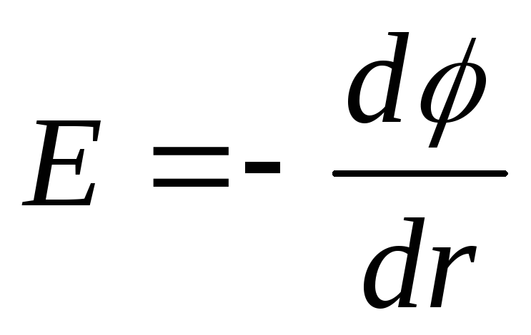
3.5. Relationship between electrostatic field strength and potential

Electric field strength - magnitude, numerically equal to strength acting on the charge. Potential is a value numerically equal to the potential energy of the charge. Thus, there must be a relationship between these quantities, similar to the relationship between potential energy and force (i.e.

). The work of the field forces on the charge on the path segment can be represented as

, and the decrease in the potential energy of the charge, which will arise in this case: . Whence from equality

we find:

or

, (21)

Where through arbitrarily chosen direction.

,

,

, (22)

Where

orts of coordinate axes, i.e., unit vectors. Vector with components

, where

scalar function of coordinates

called gradient functions and is denoted by the symbol

(or

, where is the nabla operator). So the potential gradient is:

(24)

And from (23) and (24) it follows that

(25)

Since the gradient is a vector showing the direction of the fastest change of some quantity, the value of which changes from one point in space to another, then the gradient of the potential (where r-radius-vector) is a vector directed in the direction of the most rapid increase in the potential, numerically equal to the rate of its change per unit length in this direction.

Because the

is a vector quantity, then its modulus is expressed as:

, (26)

Just like the modulus of a vector :

(27)

The “–” sign (25) indicates that the tension is directed in the direction of decreasing potential. Formula (25) allows you to find the field strength at each point from known values or solve the inverse problem, i.e., from the given values at each point, find the potential difference between two arbitrary points of the field.

3.6. Equipotential surfaces

The potential of an electrostatic field is a function that varies from point to point. However, in any real case, it is possible to single out a set of points whose potentials are the same.

G the geometric locus of points of constant potential is called a surface of equal potential or an equipotential surface.

Take a uniformly charged infinite plane (Fig. 3.6). The field created by such a plane is homogeneous, and the lines of tension are normal to the plane. It follows that the work of moving a charge from a certain point AT 1 to any other point AT 2 , located at the same distance from the charged surface as the point AT 1 equals zero. Indeed, when moving some charge q in a straight line AT 1 AT 2 the force acting on the charge from the side of the field will always be perpendicular to the displacement, and, therefore, its work is zero. But this work can be represented, on the other hand, in the form:

, (28)

G de and

are, respectively, the potentials of the points AT 1 and AT 2 . Hence, since A = 0, then =, i.e., the potentials of points equidistant from the charged plane are the same. Thus, surfaces of equal potential (equipotential surfaces) are planes parallel to the charged plane. If the plane is positively charged, then the value of the potential decreases with distance from the charged plane. It is obvious that the surfaces of equal potential are located symmetrically on both sides of the charged plane.

The equipotential surfaces of the field of a point charge are spheres with a radius r , whose center is in the center of a point charge, i.e.

(Fig. 3.7). On fig. 3.6 and fig. 3.7 the intensity vector is perpendicular to the equipotential surfaces.

Let us show that the intensity vector is perpendicular to the equipotential surface. Consider the work of moving a charge over a surface of equal potential on a small section of the path ∆ S (Fig. 3.7). At the same time, work electrical force

on this path will be:

Where α is the angle between the direction of the force f and displacement ∆ S. On the other hand, this work can be expressed as the product of the value of the moving charge and the potential difference in the initial and final positions of the charge, i.e.

.

Since the movement goes along the equipotential surface, the potential difference

and

, or cosα = 0, so α = 90 0 i.e. angle between force direction and displacement ∆ S is equal to 90 0 . But , i.e. directions and match, so the angle between and ∆ S, α=90 0 i.e. the direction of the electrostatic field vector is always perpendicular to the equipotential surface.

You can draw as many equipotential surfaces around a charged body as you like. By the density of equipotential surfaces, one can judge the value , however, provided that the potential difference between two adjacent equipotential surfaces is equal to a constant value.

The formula expresses the relationship between the potential and the strength and allows using the known values of φ to find the field strength at each point. It is also possible to solve the inverse problem, i.e. by known values at each point of the field find the potential difference between two arbitrary points of the field. To do this, we use the fact that the work done by the field forces on the charge q when moving it from point 1 to point 2 can be calculated as:

On the other hand, the work can be represented as:

, then

The integral can be taken along any line connecting point 1 and point 2, since the work of the field forces does not depend on the path.

When traversing a closed loop

we get:

those. came to the well-known theorem on the circulation of the intensity vector: the circulation of the electrostatic field strength vector along any closed loop is equal to zero.

A field with this property is called potential.

From the vanishing of the circulation of the vector it follows that the lines of the electrostatic field cannot be closed:they start on positive charges(origins )and on negative charges run out(drains )or go to infinity.

Let us generalize the Gauss theorem and the theorem on the circulation of the electrostatic field strength vector in vacuum. Since , a

, then

. Because the

(

is the Laplace operator), then for the potential φ we obtain the expression

or

, which is called Poisson equation.

This equation allows, according to the known charge distribution

and the given boundary condition for the potential φ to determine the values

at all points of the field, and then using the formula to find the tension

fields, i.e. solve the direct problem of electrostatics.

3.7. Calculation of the potential difference from the field strength of the simplest electrostatic fields

The established relationship between the strength and potential allows, by the known strength of the field, to find the potential difference between two arbitrary points of this field.

Let's consider several examples of calculating the potential difference between the points of the field created by some charged bodies.

1. The field of a uniformly charged infinite plane

The field of a uniformly charged infinite plane, found using the Ostrogradsky-Gauss theorem, is determined by the formula

, where σ is the surface charge density. Potential difference between points lying at distances x 1 and x 2 from the plane, is equal to

.

d E = 0, between the plates the potential decreases according to the logarithmic law, and the second plate (outside the cylinders) shields the electric field and φ and E are equal to zero.
Figure 3.10
On fig. 3.10 shows the dependence of tension E and capacity from r.
4. Field of a uniformly charged spherical surface
Considering examples of applying the Ostrogradsky-Gauss theorem, we found that the field strength of the sphere is determined by the formula:

(Fig. 3.11). And since

, then

Figure 3.11
. If accept r 1 = r , a r 2 =∞, then the potential outside the spherical surface is determined by the expression), is determined by the formula
By choosing the zero potential level at the point r 2 =∞ the potential of any point inside the charged ball can be found as follows:

. After integration, we get

.

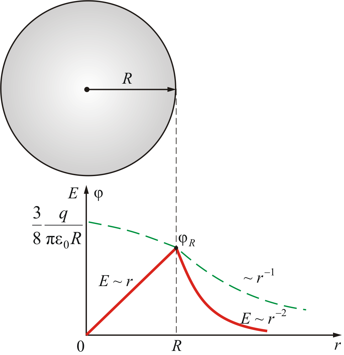
Figure 3.12
Considering that

, then

( 38 )
From the obtained relations, we can make the following conclusions .
- Using the Gauss theorem, it is relatively easy to calculate E and φ from various charged surfaces.
- The field strength in vacuum changes abruptly when passing through a charged surface.
- Field potential - always continuous function coordinates.
test questions
1. How to show that an electrostatic field is potential?
2. What is potential?
3. What is called the circulation of the tension vector?
4. What is the relationship between tension and potential? How to draw a picture of field lines from the picture of equipotential surfaces?
5. What is the work done to move a charge across an equipotential surface?
6. Give examples of calculating the potential difference of the simplest electrostatic fields.
7. How does a dipole behave in an external electrostatic field?