Electric field lines
Electric charge is a physical scalar quantity that determines the ability of bodies to be a source of electromagnetic fields and take part in electromagnetic interaction.
AT closed system the algebraic sum of the charges of all particles remains unchanged.
(... but not the number of charged particles, because there are transformations of elementary particles).
closed system
- a system of particles into which charged particles do not enter from the outside and do not go out.
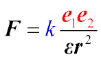
Coulomb's law
- the basic law of electrostatics.
The force of interaction of two point motionless charged bodies in vacuum is directly proportional to
the product of charge modules and is inversely proportional to the square of the distance between them.
When are bodies considered point? - if the distance between them is many times greater than the size of the bodies.
If two bodies have electric charges, then they interact according to Coulomb's law.
tension electric field. The principle of superposition. Calculation electrostatic field systems of turned charges based on the principle of superposition.
The electric field strength is a vector physical quantity that characterizes the electric field at a given point and is numerically equal to the ratio of the force acting on a stationary [trial charge placed in given point field, to the value of this charge :
The superposition principle is one of the most general laws in many branches of physics. In its simplest form, the superposition principle says:
the result of the impact on the particle of several external forces is the vector sum of these forces.
The most famous principle of superposition in electrostatics, in which he states that the strength of the electrostatic field created at a given point by a system of charges, is the sum of the strengths of the fields of individual charges.
4. Lines of tension (lines of force) of the electric field. Tension vector flow. Density of lines of force.
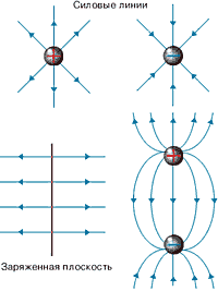
The electric field is depicted using lines of force.
Field lines indicate the direction of the force acting on a positive charge at a given point in the field.

Properties of electric field lines
Electric field lines have a beginning and an end. They start at positive charges and end in negative.
The lines of force of the electric field are always perpendicular to the surface of the conductor.
The distribution of electric field lines determines the nature of the field. The field can be radial(if the lines of force come out of one point or converge at one point), homogeneous(if the lines of force are parallel) and heterogeneous(if the lines of force are not parallel).
9.5. Electric field strength vector flow. Gauss theorem
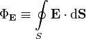
As for any vector field it is important to consider the properties of the electric field flow. The electric field flux is defined traditionally.
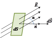
We select a small area of area Δ S, whose orientation is given by a unit normal vector (Fig. 157).
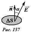
Within a small area, the electric field can be considered uniform, then the flux of the intensity vector Δ F E is defined as the product of the site area and the normal component of the intensity vector
where ![]() - scalar product of vectors and ; E n - normal to the site component of the intensity vector.
- scalar product of vectors and ; E n - normal to the site component of the intensity vector.
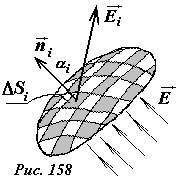
In an arbitrary electrostatic field, the flux of the intensity vector through an arbitrary surface is determined as follows (Fig. 158):
The surface is divided into small areas Δ S(which can be considered flat);
The tension vector on this site is determined (which can be considered constant within the site);
The sum of flows through all areas into which the surface is divided is calculated
This amount is called flow of the electric field strength vector through a given surface.
|
Continuous lines, the tangents to which at each point through which they pass coincide with the intensity vector, are called electric field lines or lines of tension. |
||
|
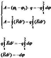
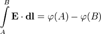
The density of lines is greater where the field strength is greater. The lines of force of the electric field created by stationary charges are not closed: they start on positive charges and end on negative ones. An electric field whose intensity is the same at all points in space is called homogeneous. The density of lines is greater near charged bodies, where the intensity is greater. The lines of force of the same field do not intersect. A force acts on any charge in an electric field. If the charge moves under the action of this force, then the electric field does work. The work of forces on the movement of a charge in an electrostatic field does not depend on the trajectory of the charge and is determined only by the position of the initial and final points. Let us consider a uniform electric field formed by flat plates charged differently. The field strength is the same at all points. Let a point charge q move from point A to point B along curve L. When the charge moves by a small amount D L, the work is equal to the product of the modulus of force by the amount of displacement and the cosine of the angle between them, or, which is the same, the product of the magnitude of the point charge by the intensity fields and onto the projection of the displacement vector onto the direction of the intensity vector. If you count full work by moving the charge from point A to point B, then it, regardless of the shape of the curve L, will turn out to be equal to work by moving the charge q along field line to point B 1 . The work of moving from point B 1 to point B is zero, since the force vector and the displacement vector are perpendicular. |
| |
5. Gauss's theorem for an electric field in vacuum
General wording: Vector flow electric field strength through any arbitrarily chosen closed surface is proportional to the enclosed inside this surface electric charge.
|
GHS |
SI |
This expression is the Gauss theorem in integral form.
Comment: the flow of the stress vector through the surface does not depend on the charge distribution (arrangement of charges) inside the surface.
In differential form, Gauss's theorem is expressed as follows:
|
GHS |
SI |
|
|
Here is the volumetric charge density (in the presence of a medium - the total density of free and bound charges), and - nabla operator.
Gauss's theorem can be proved as a theorem in electrostatics from Coulomb's law ( see below). However, the formula is also true in electrodynamics, although in it it most often does not act as a proved theorem, but acts as a postulated equation (in this sense and context it is more logical to call it Gauss law .
6. Application of the Gauss theorem to the calculation of the electrostatic field of a uniformly charged long filament (cylinder)
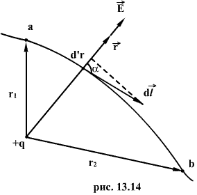
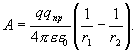
Field of a uniformly charged infinite cylinder (thread). An infinite cylinder of radius R (Fig. 6) is uniformly charged with linear densityτ (τ = –dQ/dt charge per unit length). From considerations of symmetry, we see that the lines of tension will be directed along the radii of the circular sections of the cylinder with the same density in all directions relative to the axis of the cylinder. Let us mentally construct as a closed surface a coaxial cylinder of radius r and height l. Vector flow E through the ends of the coaxial cylinder is equal to zero (the ends and lines of tension are parallel), and through the side surface it is equal to 2πr l E. Using the Gauss theorem, for r>R 2πr l E = τ l/ε 0 , whence (5) If r 7. Application of the Gauss theorem to the calculation of the electrostatic field of a uniformly charged plane Field of a uniformly charged infinite plane. The infinite plane (Fig. 1) is charged with a constant surface density+σ (σ = dQ/dS is the charge per unit surface). The tension lines are perpendicular to this plane and directed from it to each side. Let us take as a closed surface a cylinder, the bases of which are parallel to the charged plane, and the axis is perpendicular to it. Since the generatrices of the cylinder are parallel to the lines of the field strength (сosα=0), then the flux of the intensity vector through the side surface of the cylinder is equal to zero, and the total flux through the cylinder is equal to the sum of the fluxes through its bases (the areas of the bases are equal and for the base E n coincides with E), i.e. equal to 2ES. The charge enclosed inside the constructed cylindrical surface is equal to σS. According to the Gauss theorem, 2ES=σS/ε 0 , whence (1) From formula (1) it follows that E does not depend on the length of the cylinder, i.e., the field strength at any distances is equal in absolute value, in other words, the field of a uniformly charged plane uniformly. 8. Application of the Gauss theorem to the calculation of the electrostatic field of a uniformly charged sphere and a volumetrically charged ball. Field of a uniformly charged spherical surface. A spherical surface of radius R with a total charge Q is charged uniformly with surface density+σ. Because the charge is distributed uniformly over the surface, the field that it creates has spherical symmetry. This means that the lines of tension are directed radially (Fig. 3). Let's mentally draw a sphere of radius r, which has a common center with a charged sphere. If r>R,ro, the entire charge Q, which creates the considered field, gets inside the surface, and, according to the Gauss theorem, 4πr 2 E = Q/ε 0 , whence The field of a volumetrically charged sphere. A ball of radius R with a total charge Q is charged uniformly with bulk densityρ (ρ = dQ/dV is the charge per unit volume). Taking into account symmetry considerations similar to item 3, we can prove that for the field strength outside the ball the same result will be obtained as in case (3). Inside the ball, the field strength will be different. Sphere of radius r" 9. The work of the forces of the electric field when moving the charge. The theorem on the circulation of the electric field strength. The elementary work done by the force F when moving a point electric charge from one point of the electrostatic field to another on a segment of the path is, by definition, equal to where is the angle between the force vector F and the direction of motion. If the work is done by external forces, then dA0. Integrating the last expression, we get that the work against the field forces when moving the test charge from point “a” to point “b” will be equal to where is the Coulomb force acting on the test charge at each point of the field with intensity E. Then the work Let the charge move in the charge field q from point “a”, remote from q at a distance to point “b”, remote from q at a distance (Fig. 1.12). As can be seen from the figure, then we get As mentioned above, the work of the forces of the electrostatic field, performed against external forces, is equal in magnitude and opposite in sign to the work of external forces, therefore Electric field circulation theorem. tension and potential- these are two characteristics of the same object - an electric field, so there must be a functional relationship between them. Indeed, the work of the field forces on the movement of the charge q from one point in space to another can be represented in two ways: Whence it follows that This is the desired connection between the strength and potential of the electric field in differential form. Fig.2.11. Vectors
and
gradφ.
. From the property of the potentiality of the electrostatic field, it follows that the work of the field forces in a closed loop (φ 1 = φ 2) is equal to zero: so we can write The last equality reflects the essence second main theorem electrostatics - electric field circulation theorems
, according to which field circulation
along arbitrary closed loop is equal to zero. This theorem is a direct consequence
potentialities
electrostatic field. 10. Electric field potential. Relationship between potential and tension. electrostatic potential(see also Coulomb potential
) - scalar energy characteristic electrostatic field characterizing potential energy field possessed by a single charge placed at the given point in the field. Unit of measurement potential is thus a unit of measurement work, divided by the unit of measurement charge(for any system of units; more about units of measurement - see below). electrostatic potential- a special term for a possible replacement for the general term of electrodynamics scalar potential
in a particular case electrostatics(historically, the electrostatic potential appeared first, and the scalar potential of electrodynamics is its generalization). Use of the term electrostatic potential determines the presence of an electrostatic context. If such a context is already obvious, one often speaks simply of potential without qualifying adjectives. The electrostatic potential is equal to the ratio potential energy interactions charge with the field to the value of this charge: Electrostatic field strength and potential are related by the relation
or vice versa
: Here - nabla operator
, that is, on the right side of the equality there is a minus gradient potential - a vector with components equal to private derivative from the potential along the corresponding (rectangular) Cartesian coordinates, taken with the opposite sign. Using this ratio and Gauss theorem for the field strength , it is easy to see that the electrostatic potential satisfies Poisson equation. In system units SI: where is the electrostatic potential (in volts), - volumetric charge density(in pendants per cubic meter), and - vacuum (in farads per metre). 11. Energy of a system of fixed point electric charges. Energy of a system of fixed point charges. As we already know, electrostatic interaction forces are conservative; This means that the system of charges has potential energy. We will look for the potential energy of a system of two fixed point charges Q 1 and Q 2 that are at a distance r from each other. Each of these charges in the field of the other has a potential energy (we use the solitary charge potential formula): where φ 12 and φ 21 are, respectively, the potentials that are created by the charge Q 2 at the point where the charge Q 1 and the charge Q 1 at the point where the charge Q 2 is located. According to, and therefore W 1 = W 2 = W and Adding to our system of two charges sequentially the charges Q 3 , Q 4 , ... , we can prove that in the case of n fixed charges, the interaction energy of the system of point charges is equal to 12. Dipole in an electric field. Polar and non-polar molecules. Polarization of dielectrics. Polarization. Ferroelectrics. If a dielectric is placed in an external electric field, then it becomes polarized, i.e., it acquires a non-zero dipole moment pV=∑pi where p is the dipole moment of one molecule. To produce a quantitative description of the polarization of a dielectric, a vector quantity is introduced - polarization, which is defined as the dipole moment of a unit volume of the dielectric: It is known from experience that for a large class of dielectrics (with the exception of ferroelectrics, see below), the polarization P depends linearly on the field strength E. If the dielectric is isotropic and E is numerically not too large, then Ferroelectrics- dielectrics that have spontaneous (spontaneous) polarization in a certain temperature range, i.e. polarization in the absence of an external electric field. Ferroelectrics include, for example, Rochelle salt NaKC 4 H 4 O 6 4H 2 O studied in detail by I. V. Kurchatov (1903-1960) and P. P. Kobeko (1897-1954) (from which this name was obtained) and barium titanate ВаТiO 3 . Polarization of dielectrics- a phenomenon associated with a limited displacement of coupled charges in dielectric or by turning electrical dipoles, usually under the influence of an external electric field, sometimes under the influence of other external forces or spontaneously. The polarization of dielectrics is characterized by electric polarization vector
. The physical meaning of the electric polarization vector is dipole moment, per unit volume of the dielectric. Sometimes the polarization vector is briefly referred to as simply the polarization. electric dipole- an idealized electrically neutral system, consisting of point and equal in absolute value positive and negative electric charges. In other words, an electric dipole is a collection of two opposite point charges equal in absolute value, located at some distance from each other. The product of a vector drawn from a negative charge to a positive one by the absolute value of the charges is called the dipole moment: In an external electric field, a moment of forces acts on an electric dipole, which tends to rotate it so that the dipole moment turns along the direction of the field. The potential energy of an electric dipole in a (constant) electric field is (In the case of an inhomogeneous field, this means that it depends not only on the moment of the dipole - its magnitude and direction, but also on the location, the point where the dipole is located). Far from the electric dipole, its intensity electric field decreases with distance, i.e. faster than point charge (). Any generally electrically neutral system containing electric charges, in some approximation (that is, actually in dipole approximation) can be considered as an electric dipole with a moment where is the charge of the -th element, is its radius vector. In this case, the dipole approximation will be correct if the distance at which the electric field of the system is studied is large compared to its characteristic dimensions. polar substances in chemistry - substances, molecules possessed electric dipole moment. Polar substances, in comparison with non-polar ones, are characterized by a high the dielectric constant(more than 10 in the liquid phase), increased boiling temperature and melting temperature. The dipole moment usually arises due to different electronegativity constituting a molecule atoms, because of which connections in the molecule acquire polarity. However, the acquisition of a dipole moment requires not only the polarity of the bonds, but also their corresponding location in space. Molecules shaped like molecules methane or carbon dioxide, are non-polar. Polar solvents most willingly dissolve polar substances, and also have the ability solvate ions. Examples of a polar solvent are water, alcohols and other substances. 13. Electric field strength in dielectrics. electrical displacement. Gauss's theorem for the field in dielectrics. The strength of the electrostatic field, according to (88.5), depends on the properties of the medium: in a homogeneous isotropic medium, the field strength E is inversely proportional to . Tension vector E, passing through the boundary of dielectrics, undergoes an abrupt change, thereby creating inconvenience in the calculation of electrostatic fields. Therefore, it turned out to be necessary, in addition to the intensity vector, to characterize the field also electric displacement vector, which for an electrically isotropic medium, by definition, is equal to Using formulas (88.6) and (88.2), the electric displacement vector can be expressed as The unit of electrical displacement is a pendant per square meter (C / m 2). Consider what can be associated with the electric displacement vector. Bound charges appear in a dielectric in the presence of an external electrostatic field created by a system of free electric charges, i.e., in a dielectric, an additional field of bound charges is superimposed on the electrostatic field of free charges. Result field in a dielectric is described by the field strength vector E, and therefore it depends on the properties of the dielectric. Vector D describes the electrostatic field generated free charges. Bound charges arising in the dielectric, however, can cause a redistribution of free charges that create a field. Therefore, the vector D characterizes the electrostatic field created free charges(i.e., in a vacuum), but with their distribution in space, which is in the presence of a dielectric. Same as the field E, field D depicted with electric displacement lines, the direction and density of which are determined in exactly the same way as for lines of tension (see § 79). Vector lines E can begin and end on any charges - free and bound, while the lines of the vector D - only on free charges.
Through the areas of the field where the bound charges are located, the lines of the vector D pass without interruption. For arbitrary closed surfaces S flow vector D through this surface where D n- vector projection D to normal n to site d S.
Gauss theorem for electrostatic field in a dielectric: i.e., the flow of the displacement vector of the electrostatic field in the dielectric through an arbitrary closed surface is equal to the algebraic sum of the enclosed inside this surface free electric charges. In this form, the Gauss theorem is valid for an electrostatic field both for homogeneous and isotropic, and for inhomogeneous and anisotropic media. For vacuum D n
=
0 E n
(
=1), then the intensity vector flux E through an arbitrary closed surface (cf. (81.2)) is Since the sources of the field E in the medium are both free and bound charges, then the Gauss theorem (81.2) for the field E in the most general form can be written as where are, respectively, the algebraic sums of free and bound charges covered by a closed surface S.
However, this formula is unacceptable for describing the field E in a dielectric, since it expresses the properties of an unknown field E through bound charges, which, in turn, are determined by it. This once again proves the expediency of introducing the electric displacement vector. . Electric field strength in a dielectric. In accordance with superposition principle the electric field in the dielectric is vectorially composed of the external field and the field of polarization charges (Fig. 3.11). We see that the magnitude of the field strength in a dielectric is less than in a vacuum. In other words, any dielectric weakens external electric field. Fig.3.11. Electric field in a dielectric. Electric field induction , where , , that is . On the other hand, whence we find that ε
0
E 0
=
ε
0
εE and, consequently, the strength of the electric field in isotropic dielectric is: This formula reveals physical meaning permittivity and shows that the electric field strength in the dielectric is times less than in a vacuum. From here follows a simple rule: to write the formulas of electrostatics in a dielectric, it is necessary in the corresponding formulas of vacuum electrostatics next to
ascribe
.
In particular, Coulomb's law in scalar form is written as: 14. Electric capacity. Capacitors (flat, spherical, cylindrical), their capacities. The capacitor consists of two conductors (plates), which are separated by a dielectric. The capacitance of the capacitor should not be affected by the surrounding bodies, so the conductors are shaped so that the field created by the accumulated charges is concentrated in a narrow gap between the capacitor plates. This condition is satisfied by: 1) two flat plates; 2) two concentric spheres; 3) two coaxial cylinders. Therefore, depending on the shape of the plates, capacitors are divided into flat, spherical and cylindrical. Since the field is concentrated inside the capacitor, the lines of tension begin on one plate and end on the other, so the free charges that arise on different plates are equal in magnitude and opposite in sign. Under capacity capacitor is understood as a physical quantity equal to the ratio of the charge Q accumulated in the capacitor to the potential difference (φ 1 - φ 2) between its plates: (1) Find the capacitance of a flat capacitor, which consists of two parallel metal plates with an area S each, located at a distance d apart and having charges +Q and –Q. If we assume that the distance between the plates is small compared to their linear dimensions, then the edge effects on the plates can be neglected and the field between the plates can be considered uniform. It can be found using the field potential formula of two infinite parallel oppositely charged planes φ 1 -φ 2 =σd/ε 0 . Given the presence of a dielectric between the plates: Electric capacity- a characteristic of a conductor, a measure of its ability to accumulate electric charge. In the theory of electrical circuits, capacitance is the mutual capacitance between two conductors; parameter of the capacitive element of the electrical circuit, presented in the form of a two-terminal network. This capacitance is defined as the ratio of the magnitude of the electric charge to potential difference between these conductors. In system SI capacitance is measured in farads. In system GHS in centimeters. For a single conductor, the capacitance is equal to the ratio of the conductor's charge to its potential, assuming that all other conductors endlessly removed and that the potential of a point at infinity is taken equal to zero. In mathematical form, this definition has the form Where - charge, is the potential of the conductor. The capacitance is determined by the geometric dimensions and shape of the conductor and the electrical properties of the environment (its dielectric constant) and does not depend on the material of the conductor. For example, the capacitance of a conducting ball of radius R is equal to (in the SI system): where ε
0
- electrical constant, ε
- . The concept of capacitance also applies to a system of conductors, in particular, to a system of two conductors separated by dielectric or vacuum, - to capacitor. In this case mutual capacitance these conductors (capacitor plates) will be equal to the ratio of the charge accumulated by the capacitor to the potential difference between the plates. For a flat capacitor, the capacitance is: where S- the area of one lining (it is assumed that they are equal), d- the distance between the plates, ε
- relative permittivity environments between the plates, ε
0
= 8.854 10 −12 f/m - electrical constant. Capacitor(from lat. condensare- “compact”, “thicken”) - bipolar with a specific meaning containers and small ohmic conductivity; storage device charge and energy of the electric field. The capacitor is a passive electronic component. Usually consists of two plate-shaped electrodes (called facings), separated dielectric, the thickness of which is small compared to the dimensions of the plates. 15. Connection of capacitors (parallel and series) In addition to what is shown in Fig. 60 and 61, as well as in fig. 62, and the parallel connection of capacitors, in which all positive and all negative plates are connected to each other, sometimes the capacitors are connected in series, i.e., so that the negative plate 16. Electric field energy and its bulk density. Electric field energy. The energy of a charged capacitor can be expressed in terms of quantities characterizing the electric field in the gap between the plates. Let's do this using the example of a flat capacitor. Substituting the expression for capacitance into the formula for the energy of a capacitor gives Private U / d equal to the field strength in the gap; work S· d is the volume V occupied by the field. Consequently, If the field is uniform (which is the case in a flat capacitor at a distance d much smaller than the linear dimensions of the plates), then the energy contained in it is distributed in space with a constant density w. Then bulk energy density electric field is Taking into account the relation, we can write In an isotropic dielectric, the directions of the vectors D and E match and Substitute the expression , we get The first term in this expression coincides with the energy density of the field in vacuum. The second term is the energy spent on the polarization of the dielectric. Let us show this by the example of a nonpolar dielectric. The polarization of a nonpolar dielectric is that the charges that make up the molecules are displaced from their positions under the influence of an electric field E. Per unit volume of the dielectric, the work expended on the displacement of charges q i by d r i , is The expression in brackets is the dipole moment per unit volume or the polarization of the dielectric R. Consequently, . Vector P linked to vector E ratio . Substituting this expression into the formula for work, we get Having carried out the integration, we determine the work expended on the polarization of a unit volume of the dielectric Knowing the energy density of the field at each point, you can find the energy of the field enclosed in any volume V. To do this, you need to calculate the integral: 17. Direct electric current, its characteristics and conditions of existence. Ohm's law for a homogeneous section of a circuit (integral and differential forms) For the existence of a direct electric current, the presence of free charged particles and the presence of a current source are necessary. in which the conversion of any type of energy into the energy of an electric field is carried out. Current source
- a device in which any type of energy is converted into the energy of an electric field. In a current source, external forces act on charged particles in a closed circuit. The reasons for the appearance of external forces in various current sources are different. For example, in batteries and galvanic cells, external forces arise due to the flow of chemical reactions, in generators of power plants they arise when a conductor moves in a magnetic field, in photocells - when light acts on electrons in metals and semiconductors. The electromotive force of the current source
called the ratio of the work of external forces to the value of the positive charge transferred from the negative pole of the current source to the positive. b) The pattern of field lines is periodic. Along the z axis, it has a period λ pr, and along the x axis - λ pop, so the lines of force of the electric field of the E-wave are closed curves lying in the xz plane. The exception is those lines that "enter" the ideal conductor or "exit" it. They must start and end on a conductive plane. On fig. 2.2 shows a group of curves constructed by numerical integration of equation (2.12) for an angle of incidence of 45°. For clarity, the dimensionless arguments of the cotangents hz and gx, that is, the phases of the longitudinal and transverse waves at a point with the corresponding coordinate value, are plotted along the coordinate axes. On the reflecting plane, the x-coordinate and the phase of the transverse wave are zero, so the curves are plotted for gx values from 0 to π/2, that is, for an interval of 1/4 of the period. A quarter of the period from π/2 to π is also chosen for the longitudinal wave. On fig. 2.2 is an illustration, so the requirements for the accuracy of the graphical construction of the field pattern are low and the differential equation can be solved in the simplest numerical way - the Euler method of the first order. According to this method, the original differential equation is approximately replaced by a finite difference equation: Calculations start from some initial point with coordinates x 0 , z 0 . Then the independent variable z is given an increment Δz, the increment Δx is calculated and the coordinates of the next point x 1 = x 0 + Δx, z 1 = z 0 + Δz are determined. This operation is repeated cyclically with a fixed increment Δz until the values of the current coordinates reach the boundaries of the construction area. The lines of force in fig. 2.2 are constructed for six initial points, for which the phase of the longitudinal wave is the same, π/2, and the phase of the transverse wave takes values from 0.25 to 1.5. Now it is possible to depict a complete picture of the lines of force of the electric field of the E-wave arising from reflection from an ideal conductive plate. To do this, it is enough to “repeat” the constructed picture the required number of times. It is only necessary to ensure that the directions of the arrows on the lines of force of neighboring figures alternate due to the spatial periodicity of the field. The result of these actions is shown in Fig. 2.3. There is a snapshot of the E-wave field that moves along the z-axis. It is necessary to pay attention to some features of the distribution of the field. As required by the boundary conditions, the electric field lines approach the reflecting surface in the direction of the normal. In addition, the arrows on adjacent curves are directed in different directions. This is because each group of curves corresponds to one half of the wavelength. This means that in the places where two neighboring groups of curves are constructed, the vectors of the electric field strength are directed oppositely. This is easy to understand if we recall the graph of a sinusoid, on which neighboring half-waves are located on opposite sides of the coordinate axis and the function values have different signs. The same thing happens here. Along the transverse coordinate x, perpendicular to the reflecting plane, the field structure is similar. In the same figure, lines of force of the magnetic field are plotted, which are parallel to the y-axis. The direction of the magnetic field vector also changes periodically. The vector directed away from us is indicated by a solid circle, and the vector directed towards us is indicated by a circle with a dot. The diameter of the circle is proportional to the strength of the magnetic field. The magnetic field of the E-wave is concentrated in those areas of space where the transverse projection of the electric field strength is large. This is because the proportionality factor between the vectors E and H, wave resistance, in vacuum - a real value. Therefore, there is no phase shift between the electric and magnetic fields, and the positions of the maxima of their transverse components coincide. A guided E-wave occurs if the incident wave is polarized parallel and falls at an angle of less than 90°. At an angle of incidence of this wave of 90°, a guided transverse wave (T-wave) will occur. It propagates along an ideal conducting plane without reflection. This means that the transverse wave number is equal to zero, and the longitudinal one coincides with the phase coefficient of the wave in vacuum. The projections of the complex amplitudes of the electromagnetic field vectors follow directly from formulas (2.4) and (2.5), in which the coefficient 2 should be omitted, since there is no reflected wave. As a result, we get: Based on these formulas, expressions can be written for the instantaneous values of the field strength vectors at time t = 0: A snapshot of the structure of the T-wave field in the xz plane, built according to these formulas, is shown in fig. 2.4. It is no different from the field of a homogeneous plane wave in free space. The wave propagates along the z axis. The electric field lines are oriented along the x-axis, that is, vertically and perpendicular to the guide plane, and the magnetic field lines are oriented horizontally, along the y-axis. In neighboring half-waves, the vectors are directed oppositely. The technique for studying the spatial structure of the H-wave electromagnetic field over a perfectly conducting plane is similar. And the result will be similar, so let's immediately turn to Fig. 2.5, which shows a snapshot of the distribution of field lines for an angle of incidence of 45°. On the reflecting plane, the normal component of the vector H and the tangential component of the vector E turn to zero. This corresponds to the boundary conditions on the surface of an ideal conductor. Otherwise, the patterns of the fields of E- and H-waves are the same up to a permutation of the vectors E and N. Electric charge (amount of electricity) is a physical scalar quantity that determines the ability of bodies to be a source of electromagnetic fields and take part in electromagnetic interaction. Electric charge was first introduced in Coulomb's law in 1785. The unit of charge in the International System of Units (SI) is the pendant - an electric charge passing through the cross section of a conductor at a current strength of 1 A in a time of 1 s. A charge of one pendant is very large. If two charge carriers ( q 1 = q 2 = 1 C) placed in a vacuum at a distance of 1 m, then they would interact with a force of 9 10 9 H, that is, with the force with which the Earth's gravity would attract an object with a mass of about 1 million tons. The electric charge of a closed system is preserved in time and quantized - it changes in portions that are multiples of the elementary electric charge, that is, in other words, the algebraic sum of the electric charges of bodies or particles that form an electrically isolated system does not change during any processes occurring in this system. Charge interaction The simplest and most everyday phenomenon in which the fact of the existence of electric charges in nature is revealed is the electrification of bodies upon contact. The ability of electric charges to both mutual attraction and mutual repulsion is explained by the existence of two different types of charges. One kind of electric charge is called positive, and the other is called negative. Oppositely charged bodies attract each other, and similarly charged bodies repel each other. When two electrically neutral bodies come into contact, as a result of friction, charges pass from one body to another. In each of them, the equality of the sum of positive and negative charges is violated, and the bodies are charged differently. When a body is electrified through influence, the uniform distribution of charges is disturbed in it. They are redistributed so that in one part of the body there is an excess of positive charges, and in another - negative. If these two parts are separated, then they will be charged differently. The law of conservation of email. charge In the system under consideration, new electrically charged particles can form, for example, electrons - due to the phenomenon of ionization of atoms or molecules, ions - due to the phenomenon of electrolytic dissociation, etc. However, if the system is electrically isolated, then the algebraic sum of the charges of all particles, including again appearing in such a system is always equal to zero. The law of conservation of electric charge is one of the fundamental laws of physics. It was first experimentally confirmed in 1843 by the English scientist Michael Faraday and is currently considered one of the fundamental laws of conservation in physics (similar to the laws of conservation of momentum and energy). Increasingly sensitive experimental tests of the law of conservation of charge, which continue to this day, have not yet revealed deviations from this law. .
Electric charge and its discreteness. The law of conservation of charge. The law of conservation of electric charge states that the algebraic sum of the charges of an electrically closed system is conserved. q, Q, e are designations of electric charge. Units of charge in SI [q]=Cl (Coulomb). 1mC = 10-3 C; 1 µC = 10-6 C; 1nC = 10-9 C; e = 1.6∙10-19 C is the elementary charge. The elementary charge, e is the minimum charge found in nature. Electron: qe = - e - electron charge; m = 9.1∙10-31 kg is the mass of the electron and positron. Positron, proton: qp = + e is the charge of the positron and proton. Any charged body contains an integer number of elementary charges: q = ± Ne; (1) Formula (1) expresses the discreteness principle of electric charge, where N = 1,2,3… is a positive integer. The law of conservation of electric charge: the charge of an electrically isolated system does not change over time: q = const. Coulomb's law- one of the basic laws of electrostatics, which determines the force of interaction between two point electric charges. The law was established in 1785 by Sh. Coulomb with the help of the torsion scales invented by him. Coulomb was interested not so much in electricity as in the manufacture of appliances. Having invented an extremely sensitive device for measuring force - a torsion balance, he was looking for ways to use it. For suspension, the Pendant used a silk thread 10 cm long, which rotated 1 ° at a force of 3 * 10 -9 gf. With the help of this device, he established that the force of interaction between two electric charges and between two poles of magnets is inversely proportional to the square of the distance between the charges or poles. Two point charges interact with each other in a vacuum with a force
F
, the value of which is proportional to the product of charges
e
1
and
e
2
and inversely proportional to the square of the distance
r
between them:
Proportionality factor k depends on the choice of the system of units of measurements (in the system of Gaussian units k= 1, in SI ε
0
is the electrical constant). Strength F
is directed along a straight line connecting the charges, and corresponds to attraction for unlike charges and repulsion for like charges. If the interacting charges are in a homogeneous dielectric, with permittivity ε
, then the force of interaction decreases in ε
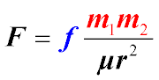
once: Coulomb's law is also called the law that determines the strength of the interaction of two magnetic poles: where m
1
and m
2
- magnetic charges, μ
is the magnetic permeability of the medium, f
is the coefficient of proportionality, depending on the choice of the system of units. Electric field- a separate form of manifestation (along with the magnetic field) of the electromagnetic field. During the development of physics, there were two approaches to explaining the causes of the interaction of electric charges. According to the first version, the force action between separate charged bodies was explained by the presence of intermediate links that transmit this action, i.e. the presence of the environment surrounding the body, in which the action is transmitted from point to point with a finite speed. This theory is called short range theory
. According to the second version, the action is transmitted instantly over any distance, while the intermediate medium may be completely absent. One charge instantly "feels" the presence of another, while no changes occur in the surrounding space. This theory has been called long-range theory
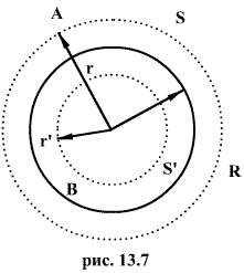
. The concept of "electric field" was introduced by M. Faraday in the 30s of the XIX century. According to Faraday, each charge at rest creates an electric field in the surrounding space. The field of one charge acts on another charge and vice versa (the concept of short-range action). An electric field created by stationary charges that does not change with time is called electrostatic. The electrostatic field characterizes the interaction of fixed charges. Electric field strength- a vector physical quantity characterizing the electric field at a given point and numerically equal to the ratio of the force acting on a fixed point charge placed at a given point of the field to the value of this charge: This definition shows why the strength of the electric field is sometimes called the power characteristic of the electric field (indeed, the difference from the vector of the force acting on a charged particle is only in a constant factor). At each point in space at a given moment of time there is its own value of the vector (generally speaking, it is different at different points in space), so this is a vector field. Formally, this is expressed in the notation representing the electric field strength as a function of spatial coordinates (and time, since it can change over time). This field, together with the field of the magnetic induction vector, is an electromagnetic field, and the laws to which it obeys are the subject of electrodynamics. The strength of an electric field in the International System of Units (SI) is measured in volts per meter [V/m] or in newtons per pendant [N/C]. The force with which an electromagnetic field acts on charged particles[ The total force with which an electromagnetic field (generally including electric and magnetic components) acts on a charged particle is expressed by the Lorentz force formula: where q- the electric charge of the particle, - its speed, - the vector of magnetic induction (the main characteristic of the magnetic field), the oblique cross denotes the vector product. The formula is given in SI units. The charges that create an electrostatic field can be distributed in space either discretely or continuously. In the first case, the field strength: n E = Σ Ei₃ i=t, where Ei is the field strength at a certain point in space, created by one i-th charge of the system, and n is the total number of discreet charges that are part of the system. An example of solving a problem based on the principle of superposition of electric fields. So, to determine the intensity of the electrostatic field, which is created in vacuum by stationary point charges q₁, q₂, …, qn, we use the formula: n E = (1/4πε₀) Σ (qi/r³i)ri i=t, where ri is the radius vector drawn from the point charge qi to the considered point of the field. Let's take another example. Determination of the strength of the electrostatic field, which is created in vacuum by an electric dipole. An electric dipole is a system of two equal in absolute value and, at the same time, opposite in sign charges q>0 and –q, the distance I between which is relatively small compared to the distance of the points under consideration. The arm of the dipole will be called the vector l, which is directed along the axis of the dipole to the positive charge from the negative one and is numerically equal to the distance I between them. The vector pₑ = ql is the electric moment of the dipole. The strength E of the dipole field at any point: E = E₊ + E₋, where E₊ and E₋ are the field strengths of electric charges q and –q. Thus, at point A, which is located on the dipole axis, the dipole field strength in vacuum will be equal to E = (1/4πε₀)(2pₑ/r³) At point B, which is located on the perpendicular restored to the dipole axis from its middle: E = (1/4πε₀)(pₑ/r3) The principle of superposition of electric fields consists of two statements: The Coulomb force of the interaction of two charges does not depend on the presence of other charged bodies. Let us assume that the charge q interacts with the system of charges q1, q2, . . . , qn. If each of the charges of the system acts on the charge q with the force F₁, F₂, ..., Fn, respectively, then the resulting force F applied to the charge q from the side of this system is equal to the vector sum of the individual forces: F = F₁ + F₂ + ... + Fn. Thus, the principle of superposition of electric fields allows us to come to one important statement. The electric field is depicted using lines of force. Field lines indicate the direction of the force acting on a positive charge at a given point in the field. Electric field lines have a beginning and an end. They start with positive charges and end with negative ones. The lines of force of the electric field are always perpendicular to the surface of the conductor. The distribution of electric field lines determines the nature of the field. The field can be radial(if the lines of force come out of one point or converge at one point), homogeneous(if the lines of force are parallel) and heterogeneous(if the lines of force are not parallel). charge density- this is the amount of charge per unit length, area or volume, thus determining the linear, surface and volume charge densities, which are measured in the SI system: in Coulombs per meter (C / m), in Coulombs per square meter (C / m² ) and Coulomb per cubic meter (C/m³), respectively. Unlike the density of matter, the charge density can have both positive and negative values, this is due to the fact that there are positive and negative charges. Linear, surface and bulk charge densities are usually denoted by the functions , and, accordingly, where is the radius vector. Knowing these functions, we can determine the total charge: Let us define the vector flow through an arbitrary surface dS, is the normal to the surface. α is the angle between the normal and the force line of the vector. You can enter an area vector. VECTOR FLOW called the scalar value Ф E equal to the scalar product of the intensity vector by the area vector For a uniform field For an inhomogeneous field where is a projection, is a projection. In the case of a curved surface S, it must be divided into elementary surfaces dS, calculate the flow through the elementary surface, and the total flow will be equal to the sum or in the limit of the integral of the elementary flows where is the integral over a closed surface S (for example, over a sphere, cylinder, cube, etc.) The flux of a vector is an algebraic quantity: it depends not only on the configuration of the field, but also on the choice of direction. For closed surfaces, the outer normal is taken as the positive direction of the normal, i.e. a normal pointing outward of the area covered by the surface. For a uniform field, the flux through a closed surface is zero. In the case of an inhomogeneous field 3. Intensity of the electrostatic field created by a uniformly charged spherical surface. Let a spherical surface of radius R (Fig. 13.7) bear a uniformly distributed charge q, i.e. the surface charge density at any point on the sphere will be the same. We enclose our spherical surface in a symmetric surface S with radius r>R. The intensity vector flux through the surface S will be equal to According to the Gauss theorem Consequently Comparing this relation with the formula for the field strength of a point charge, we can conclude that the field strength outside the charged sphere is as if the entire charge of the sphere were concentrated in its center. 2. Electrostatic field of the ball. Let we have a ball of radius R, uniformly charged with bulk density. At any point A, lying outside the ball at a distance r from its center (r> R), its field is similar to the field of a point chargelocated at the center of the ball. Then outside the ball and on its surface (r=R)
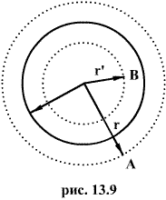
![]() (3) For r>R, the field decreases with distance r according to the same law as for point charge. The plot of E versus r is shown in fig. 4. If r"
(3) For r>R, the field decreases with distance r according to the same law as for point charge. The plot of E versus r is shown in fig. 4. If r" 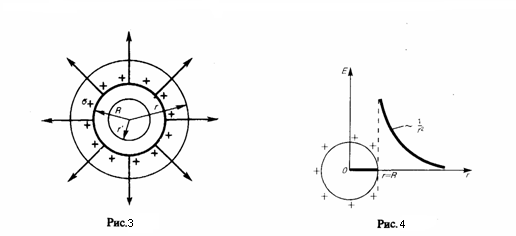
![]()


![]()
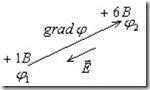
![]() - a vector directed from a point with a lower potential to a point with a higher potential (Fig. 2.11).
- a vector directed from a point with a lower potential to a point with a higher potential (Fig. 2.11).![]() ,
, ![]() .
.
![]() (1) where φ i is the potential that is created at the point where the charge Q i is located, by all charges, except for the i-th one.
(1) where φ i is the potential that is created at the point where the charge Q i is located, by all charges, except for the i-th one.![]()
![]() (89.3)
(89.3)![]()
![]()
![]() or in absolute terms
or in absolute terms![]()
![]() (2) where ε is the permittivity. Then from formula (1), replacing Q=σS, taking into account (2), we find an expression for the capacitance of a flat capacitor: (3) To determine the capacitance of a cylindrical capacitor, which consists of two hollow coaxial cylinders with radii r 1 and r 2 (r 2 > r 1), one is inserted into the other, again neglecting edge effects, we consider the field to be radially symmetric and acting only between cylindrical plates. The potential difference between the plates is calculated by the formula for the potential difference of the field of a uniformly charged infinite cylinder with a linear density τ =Q/ l (l- the length of the plates). In the presence of a dielectric between the plates, the potential difference (4) Substituting (4) into (1), we find the expression for the capacitance of a cylindrical capacitor: (5) To find the capacitance of a spherical capacitor, which consists of two concentric plates separated by a spherical dielectric layer, we use the formula for potential difference between two points lying at distances r 1 and r 2 (r 2 > r 1) from the center of a charged spherical surface. In the presence of a dielectric between the plates, the potential difference (6) Substituting (6) into (1), we obtain
(2) where ε is the permittivity. Then from formula (1), replacing Q=σS, taking into account (2), we find an expression for the capacitance of a flat capacitor: (3) To determine the capacitance of a cylindrical capacitor, which consists of two hollow coaxial cylinders with radii r 1 and r 2 (r 2 > r 1), one is inserted into the other, again neglecting edge effects, we consider the field to be radially symmetric and acting only between cylindrical plates. The potential difference between the plates is calculated by the formula for the potential difference of the field of a uniformly charged infinite cylinder with a linear density τ =Q/ l (l- the length of the plates). In the presence of a dielectric between the plates, the potential difference (4) Substituting (4) into (1), we find the expression for the capacitance of a cylindrical capacitor: (5) To find the capacitance of a spherical capacitor, which consists of two concentric plates separated by a spherical dielectric layer, we use the formula for potential difference between two points lying at distances r 1 and r 2 (r 2 > r 1) from the center of a charged spherical surface. In the presence of a dielectric between the plates, the potential difference (6) Substituting (6) into (1), we obtain ![]()
![]()
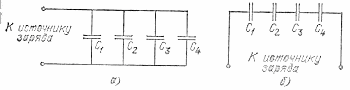 Rice. 62. Connection of capacitors: a) parallel; b) sequential the first capacitor was connected to the positive plate of the second, the negative plate of the second - to the positive plate of the third, etc. (Fig. 62, b). In the case of a parallel connection, all capacitors are charged to the same potential difference U, but the charges on them may be different. If their capacitances are equal to C1, C2, ..., Cn, then the corresponding charges will be The total charge on all capacitors and, therefore, the capacitance of the entire system of capacitors (35.1) So, the capacitance of a group of capacitors connected in parallel is equal to the sum of the capacitances of individual capacitors. In the case of capacitors connected in series (Fig. 62, b), the charges on all capacitors are the same. Indeed, if we place, for example, a charge +q on the left plate of the first capacitor, then due to induction, a charge -q will appear on its right plate, and a charge +q will appear on the left plate of the second capacitor. The presence of this charge on the left plate of the second capacitor, again due to induction, creates a charge -q on its right plate, and a charge + q on the left plate of the third capacitor, etc. Thus, the charge of each of the capacitors connected in series is equal to q. The voltage on each of these capacitors is determined by the capacitance of the corresponding capacitor: where Ci is the capacitance of one capacitor. The total voltage between the extreme (free) plates of the entire group of capacitors Therefore, the capacitance of the entire system of capacitors is determined by the expression
 ![]() (35.2) From this formula it can be seen that the capacitance of a group of capacitors connected in series is always less than the capacitance of each of these capacitors individually.
(35.2) From this formula it can be seen that the capacitance of a group of capacitors connected in series is always less than the capacitance of each of these capacitors individually.![]()
![]()
![]()

![]()
Electric field lines
Properties of electric field lines

§5 The flow of the intensity vector
![]()
![]()
![]()

![]()
![]()

![]()


