Graphic representation of fields. Graphical method for depicting the structure of electric fields. lines of force

Properties physical bodies and objects are described physical quantities . One of these quantities for electric field is tension. In accordance with the previously formulated definition, it describes the force action of the field on charged bodies at a certain point in the electric field. If the field is inhomogeneous, then the intensity in different points fields are different. And in order to describe the properties of the field at many points, it is necessary to submit a large number of intensity values. This complicates the study of the field and prevents the creation in the human imagination of the idea of the field in each specific case.

The strength of the electric field is its power characteristic.

It helps to better represent the structure of the electric field graphic method. At the heart of the graphical presentation method electric field structures lie real phenomena that can be observed in experiments.

Let a small particle of a substance, also having a positive charge, be introduced into the electric field of a positively charged ball. If this particle is free and the action of the gravitational field is insignificant, then under the influence of an electric force it will move away from the ball. Similar will be observed at any point in the field of a charged ball (Fig. 4.20).

Having depicted the trajectories of motion of many positively charged particles in an electric field, and indicating the direction to them operating force, we get a picture called spectrum this field.

The lines that form the spectrum of the electric field are called lines of tension electric field, or power lines.

concept field line was first introduced into science by M. Faraday on the basis of knowledge gained in the course of experimental research.

Experiments known to M. Faraday can be carried out in modern conditions.

Let's take a metal conductor with paper strips attached to it and connect it to the conductor of the electrophore machine. If we put it into action, then all the strips of paper will diverge in different directions due to mutual repulsion (Fig. 4.21). The results of this experiment (and others like it) make it possible to construct the spectrum of the electric field of a single charged body. It is shown in fig. 4.22. The arrows on the lines of force show the direction of the force that will act on a positively charged body located at a given point in the field.

Therefore, the lines of force "leave" a positively charged body and "enter" a negatively charged body (Fig. 4.22). It should be remembered that they "exit" and "enter" perpendicular to the surface of the body.

The lines of electric field strength are perpendicular to the surface of a charged body at the points where they begin.Material from the site

Let's take two metal conductors with paper strips and connect them to the conductors of the electrophore machine. We set the electrophore machine in action and we will see that the paper strips will begin to attract each other (Fig. 4.23). Accordingly, the field of two oppositely charged bodies will have the spectrum shown in fig. 4.24.

The curvilinear shape of the lines of tension is explained by the fact that two forces act on a positively charged particle from the side of each body. The resultant of these forces at each point of the field is tangent to the lines of tension.

Lines tangent to which at any point show the direction of the force acting on a positively charged point body are called power lines.

The directions of the forces that will act at different points in the field of two charged bodies are shown in fig. 4.25.

Since the lines of tension are always perpendicular to the surface, the spectra of the fields of bodies of various shapes will be different (Fig. 4.26).

On this page, material on the topics:

Spectra el. fields of various charged bodies
Graphic image of the electric field abstract
Images of electric field lines in experiments
a b

Knowing the intensity vector of the electrostatic field at each of its points, this field can be visualized with the help of force lines of intensity (lines of the vector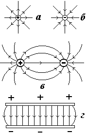 ). lines of force tensions are drawn so that the tangent to them at each point coincides with the direction of the tension vector (Fig. 1.4, a).
The number of lines penetrating a single area dS, perpendicular to them, is drawn in proportion to the modulus of the vector (Fig. 1.4, b).
The lines of force are assigned a direction coinciding with the direction of the vector . The resulting pattern of the distribution of lines of tension makes it possible to judge the configuration of a given electric field at its different points. Field lines start at positive charges and terminate in negative charges. On fig. 1.5 shows the lines of tension of point charges (Fig. 1.5, a, b); systems of two opposite charges (Fig. 1.5, in) - an example of an inhomogeneous electrostatic field and two parallel oppositely charged planes (Fig. 1.5, G) is an example of a uniform electric field.
1.5. Charge distribution
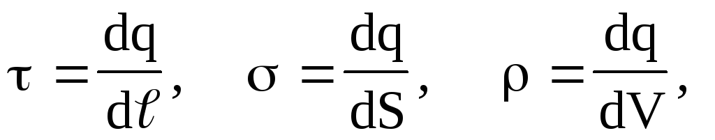
In some cases, to simplify mathematical calculations, it is convenient to replace the true distribution of discrete point charges with a fictitious continuous distribution. In the transition to a continuous distribution of charges, the concept of charge density is used - linear , surface  and volumetric , i.e.

(1.12)
where dq is the charge distributed accordingly over the element of length

, surface element dS and volume element dV.
With these distributions taken into account, formula (1.11) can be written in a different form. For example, if the charge is distributed over the volume, then instead of q i you need to use dq = dV, and replace the sum symbol with an integral, then

. (1.13)
1.6. electric dipole
To explain the phenomena associated with charges in physics, the concept is used electric dipole.
A system of two equal in magnitude opposite point charges, the distance between which is much less than the distance to the studied points in space, is called an electric dipole. According to the definition of a dipole, +q=q= q.

A straight line connecting opposite charges (poles) is called the dipole axis; point 0 - the center of the dipole (Fig. 1.6). The electric dipole is characterized dipole arm: vector , directed from a negative charge to a positive one. The main characteristic of a dipole is electric dipole moment = q . (1.14)
By absolute value
p = q . (1.15)
In SI, the electric dipole moment is measured in coulombs times a meter (C m).
Let us calculate the potential and strength of the electric field of the dipole, considering it to be a point, if  r.
Potential of an electric field created by a system of point charges at an arbitrary point characterized by a radius vector , we write in the form:

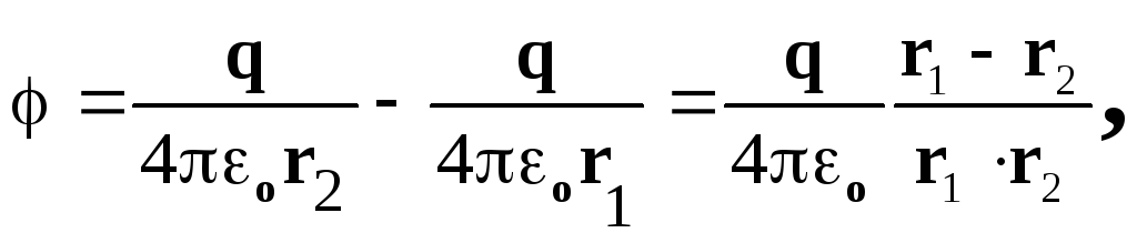
where r 1 r 2  r 2 , r 1  r 2  r =

, because  r;   angle between radius vectors and (Fig. 1.6) . With this in mind, we get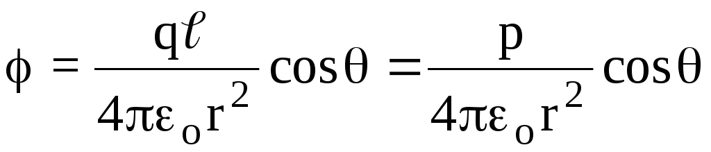

. (1.16)
Using the formula relating the potential gradient to the intensity, we find the intensity created by the electric field of the dipole. Let's decompose the vector electric dipole field into two mutually perpendicular components, i.e.

(Fig. 1. 6).
The first of them is determined by the movement of a point characterized by the radius vector (for a fixed value of the angle ), i.e., we find the value of E  by differentiation (1.81) with respect to r, i.e.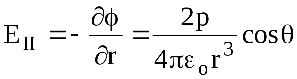

. (1.17)
The second component is determined by the movement of the point associated with a change in the angle  (for a fixed r), i.e. E  we find by differentiating (1.16) with respect to :

, (1.18)
where

,d = rd.
The resulting tension E 2 \u003d E  2 + E  2 or after substitution

. (1.19)
Comment: At  = 90 o

, (1.20)
i.e., the intensity at a point on a straight line passing through the center of the dipole (i.e. O) and perpendicular to the axis of the dipole.
When  = 0 about

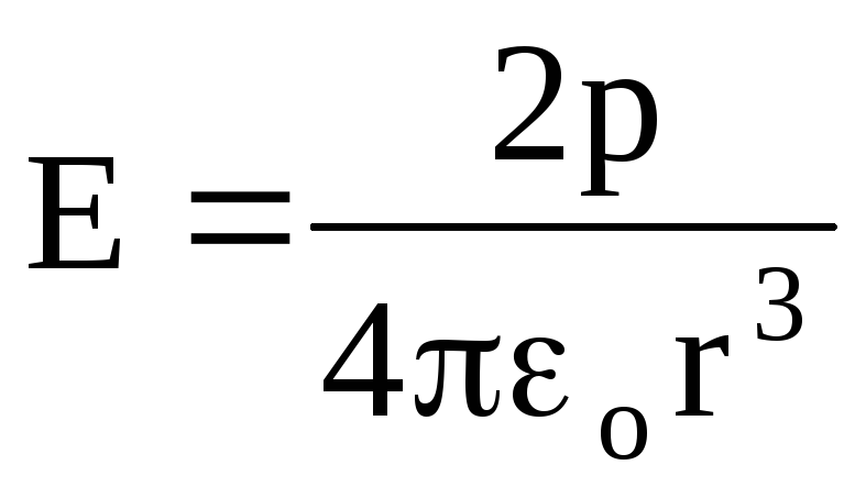, (1.21)
i.e., at a point on the continuation of a straight line coinciding with the axis of the dipole.
An analysis of formulas (1.19), (1.20), (1.21) shows that the dipole electric field strength decreases with distance in inverse proportion to r 3 , i.e. faster than for a point charge (inversely proportional to r 2).

For greater clarity, the electric field is often depicted using lines of force and equipotential surfaces.
lines of force – these are continuous lines, the tangents to which at each point through which they pass coincide with the electric field strength vector (Fig. 1.5). The density of field lines (the number of field lines passing through a unit area) is proportional to the electric field strength.
Equipotential surfaces (equipotentials) – surfaces of equal potential. These are surfaces (lines) when moving along which the potential does not change. Otherwise, the potential difference between any two points of the equipotential surface is equal to zero. The lines of force are perpendicular to the equipotential surfaces and directed in the direction of the sharpest decrease in the potential. This fact follows from equation (1.10) and is proved in the course of mathematical analysis, section "Scalar and vector fields".
Consider, as an example, an electric field generated at a distance from a point charge. According to (1.11,b), the intensity vector coincides with the direction of the vector if the charge is positive and opposite if the charge is negative. Consequently, the lines of force diverge radially from the charge (Fig. 1.6, a, b). The density of field lines, like the intensity, is inversely proportional to the square of the distance (

) to charge. The equipotential surfaces of the electric field of a point charge are spheres centered at the location of the charge.

On fig. 1.7 shows the electric field of a system of two equal in absolute value, but opposite in sign, point charges. We leave this example to the readers to analyze on their own. We only note that lines of force always begin on positive charges and end on negative ones. In the case of an electric field of one point charge (Fig. 1.6, a, b), it is assumed that the lines of force break off at very distant charges of the opposite sign. It is believed that the universe as a whole is neutral. Therefore, if there is a charge of one sign, then somewhere there will definitely be a charge of the other sign equal to it in absolute value.
1.6. Gauss's theorem for an electric field in vacuum
The main task of electrostatics is the problem of finding the strength and potential of the electric field at each point in space. In Section 1.4 we solved the problem of the field of a point charge and also considered the field of a system of point charges. In this section, we will focus on a theorem that allows us to calculate the electric field of more complex charged objects. For example, a charged long thread (straight line), a charged plane, a charged sphere, and others. Having calculated the electric field strength at each point in space, using equations (1.12) and (1.13), one can calculate the potential at each point or the potential difference between any two points, i.e. solve the basic problem of electrostatics.
For a mathematical description, we introduce the concept of the flow of the intensity vector or the flow of the electric field. Flux (F) vector electric field across a flat square surface

quantity is called:

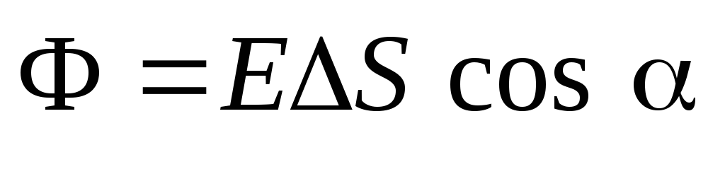, (1.16)

where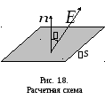 is the electric field strength, which is assumed to be constant within the site

;

is the angle between the direction of the vector and unit normal vector to the site

(Fig. 1.8). Formula (1.16) can be written using the concept of the scalar product of vectors:

. (1.15a)
In case the surface not flat, to calculate the flow it must be divided into small parts

, which can be approximately considered flat, and then write down the expression (1.16) or (1.16, a) for each piece of the surface and add them. In the limit when the surface S i very small (

), such a sum is called a surface integral and denoted

. Thus, the flow of the electric field strength vector through an arbitrary surface is defined by the expression:

. (1.17)
As an example, consider a sphere of radius , centered on a positive point charge , and determine the electric field flux through the surface of this sphere. The lines of force (see, for example, Fig. 1.6, a) emerging from the charge are perpendicular to the surface of the sphere, and at each point of the sphere, the field strength module is the same

.
Sphere area

,
then

.
Value

and represents the flow of the electric field through the surface of the sphere. Thus, we get

. It can be seen that the flux through the surface of the sphere of the electric field does not depend on the radius of the sphere, but depends only on the charge itself . Therefore, if you draw a series of concentric spheres, then the flow of the electric field through all these spheres will be the same. Obviously, the number of lines of force crossing these spheres will also be the same. We agreed to take the number of lines of force emerging from the charge equal to the flow of the electric field:

.
If the sphere is replaced by any other closed surface, then the flow of the electric field and the number of lines of force crossing it will not change. In addition, the flow of the electric field through a closed surface, and hence the number of lines of force penetrating this surface, is equal to

not only for the field of a point charge, but also for the field created by any set of point charges, in particular, by a charged body. Then the value should be considered as the algebraic sum of the entire set of charges located inside a closed surface. This is the essence of the Gauss theorem, which is formulated as follows:
The flow of the electric field strength vector through an arbitraryclosed surface equals

, where

 algebraic the amount of charges enclosedinside this surface.
Mathematically, the theorem can be written as

. (1.18)
Note that if on some surface S vector constant and parallel to vector , then the flow through such a surface. Transforming the first integral, we first took advantage of the fact that the vectors and parallel, which means

. Then took out the value for the sign of the integral due to the fact that it is constant at any point of the sphere . Applying the Gauss theorem for solving specific problems, specifically as an arbitrary closed surface, they try to choose a surface for which the conditions described above are satisfied.
We give several examples of the application of the Gauss theorem.
Example 1.2. Calculate the electric field strength of a uniformly charged infinite filament. Determine the potential difference between two points in such a field.
Solution. Assume for definiteness that the thread is positively charged. Due to the symmetry of the problem, it can be argued that the lines of force will be straight lines radially diverging from the axis of the thread (Fig. 1.9), the density of which decreases with distance from the thread according to some law. According to the same law, the magnitude of the electric field will also decrease . Equipotential surfaces will be cylindrical surfaces with an axis coinciding with the thread.
Let the charge per unit length of the thread be . This value is called the linear charge density and is measured in SI units [C/m]. To calculate the field strength, we apply the Gauss theorem. For this, as an arbitrary closed surface choose a cylinder of radius and length , whose axis coincides with the thread (Fig. 1.9). Let us calculate the electric field flux through the surface area of the cylinder. The total flow is the sum of the flow through side surface cylinder and flow through the bases
However,

, since at any point on the bases of the cylinder

. It means that

at these points. Flow through the side surface

. By Gauss's theorem, this total flow is equal to

. Thus, we got

.
The sum of the charges inside the cylinder is expressed in terms of the linear charge density :

. Given that

, we get

,

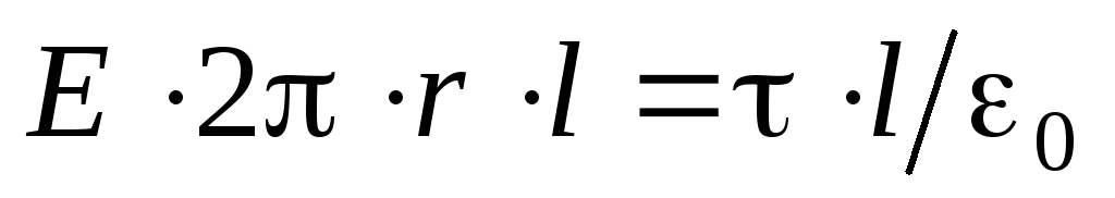, (1.19)
those. the intensity and density of the electric field lines of a uniformly charged infinite filament decreases inversely with the distance (

).
Find the potential difference between points located at distances and from the thread (belonging to equipotential cylindrical surfaces with radii and ). To do this, we use the connection between the electric field strength and the potential in the form (1.9, c):

. Taking into account expression (1.19), we obtain a differential equation with separable variables:

.

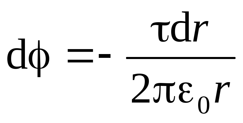
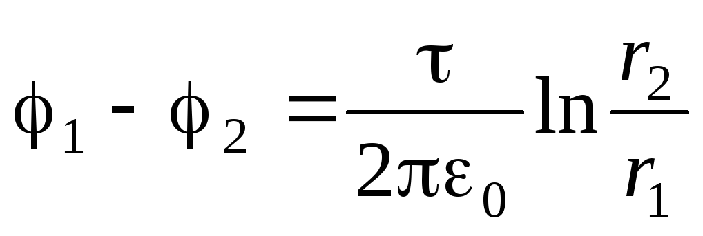Example 1.3. Calculate the electric field strength of a uniformly charged plane. Determine the potential difference between two points in such a field.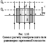
Solution. The electric field of a uniformly charged plane is shown in fig. 1.10. Due to symmetry, the lines of force must be perpendicular to the plane. Therefore, we can immediately conclude that the line density, and, consequently, the electric field strength will not change with distance from the plane. Equipotential surfaces are planes parallel to a given charged plane. Let the charge per unit area of the plane be . This value is called the surface charge density and is measured in SI in units of [C/m 2 ].
Let's apply the Gauss theorem. For this, as an arbitrary closed surface choose a cylinder with a length , whose axis is perpendicular to the plane, and the bases are equidistant from it (Fig. 1.10). Total Electric Field Flux

. The flow through the side surface is zero. The flow through each of the bases is

, that's why

. According to the Gauss theorem, we get:

.
The sum of the charges inside the cylinder , we find through the surface charge density :

. Then from where:

. (1.20)
It can be seen from the obtained formula that the field strength of a uniformly charged plane does not depend on the distance to the charged plane, i.e. at any point in space (in one half-plane) is the same both in absolute value and in direction. Such a field is called homogeneous. lines of force homogeneous field parallel, their density does not change.
Let us find the potential difference between two points of a homogeneous field (belonging to the equipotential planes and lying in one half-plane relative to the charged plane (Fig. 1.10)). Let's direct the axis vertically upwards, then the projection of the tension vector on this axis is equal to the modulus of the tension vector

. We use equation (1.9):

.
Constant value (the field is homogeneous) can be taken out from under the integral sign:

. Integrating, we get: . So, the potential of a homogeneous field depends linearly on the coordinate.
The potential difference between two points of the electric field is the voltage between these points ( ). Let us denote the distance between the equipotential planes

. Then we can write that in a uniform electric field:

. (1.21)
We emphasize once again that when using formula (1.21), we must remember that the quantity - not the distance between points 1 and 2, but the distance between the equipotential planes to which these points belong.
Example 1.4. Calculate the electric field strength of two parallel planes uniformly charged with surface charge densities

and

.
Solution. Let us use the result of Example 1.3 and the principle of superposition. According to this principle, the resulting electric field at any point in space

, where and - electric field strengths of the first and second planes. In the space between the vector planes and directed in one direction, so the modulus of the resulting field strength. In the outer space of the vector and directed in different directions, therefore (Fig. 1.11). Thus, the electric field exists only in the space between the planes. It is homogeneous, since it is the sum of two homogeneous fields.
Example 1.5. Find the strength and potential of the electric field of a uniformly charged sphere. The total charge of the sphere is , and the radius of the sphere is .
Solution. Due to the symmetry of the charge distribution, the lines of force must be directed along the radii of the sphere.
Consider a region inside a sphere. As an arbitrary surface choose a sphere of radius

, whose center coincides with the center of the charged sphere. Then the flow of the electric field through the sphere S:

. The sum of the charges inside the sphere radius is equal to zero, since all charges are located on the surface of a sphere of radius

. Then by the Gauss theorem:

. Because the

, then

. Thus, there is no field inside a uniformly charged sphere.
Consider a region outside the sphere. As an arbitrary surface choose a sphere of radius

, whose center coincides with the center of the charged sphere. The flow of an electric field through a sphere :

. The sum of the charges inside the sphere is equal to the total charge charged sphere of radius . Then by the Gauss theorem:

. Given that

, we get:

.
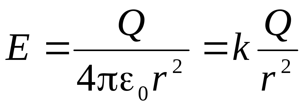Let's calculate the potential of the electric field. It is more convenient to start from the outer area

, since we know that at an infinite distance from the center of the sphere, the potential is assumed to be zero. Using equation (1.11, a) we obtain a differential equation with separable variables:

.
Constant

, because the

at

. Thus, in outer space (

):

.
Points on the surface of a charged sphere (

) will have the potential

.
Consider the area

. In this region

, therefore, from equation (1.11, a) we obtain:

. Due to the continuity of the function

constant must be equal to the value of the potential on the surface of the charged sphere:

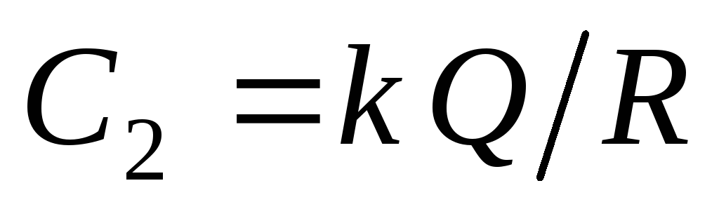. So the potential at all points inside the sphere is:

.

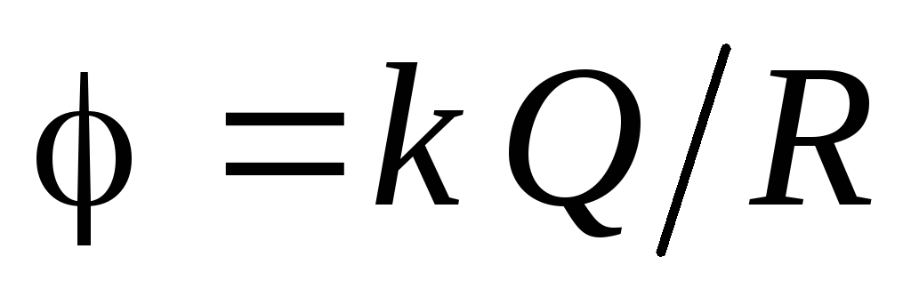So, we have obtained that the strength and potential of the electric field created by a uniformly charged sphere outside the sphere are equal to the strength and potential of the field created by point charge the same size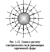 , which is the charge of the sphere placed at the center of the sphere. There is no field in the inner space, and the potential is the same at all points. The electric field (field lines and equipotential surfaces) of a charged sphere is shown in fig. 1.12. The sphere is assumed to be positively charged. Outside the sphere, the lines of force and are distributed in space in exactly the same way as the lines of force of a point charge.

On fig. 1.13 shows dependency graphs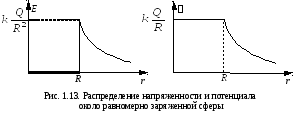

and

. Function

is continuous, and the function

changes abruptly when passing through the boundary of a charged sphere. The jump value is

. Indeed, near the charged sphere (

) field strength in outer space

, while inside it is equal to zero.
The magnitude of the jump can be expressed in terms of the surface charge density on the sphere:

.
Note that this common property electrostatic field: on a charged surface, the projection of the intensity on the direction of the normal always experiences a jump

regardless of surface shape. We recommend checking this principle for the field of a uniformly charged plane and the field of two parallel charged planes (examples 1.3, 1.4).
From the point of view of mathematics, the continuity of the potential at the points of the charged surface means that

. From the point of view of physics, the continuity of the function

can be explained as follows. If the potential at the boundary of a certain region would have a jump (discontinuity), then with an infinitely small displacement of a certain charge from point 1, lying on one side of the boundary, to point 2, lying on its other side, finite work would be done

, where and  potentials of points 1 and 2, respectively, and the value

is equal to the potential jump at the boundary of the region. The final work done on an infinitely small displacement means that infinitely large forces would act on the interface, which is impossible.
The strength of the electric field, in contrast to the potential, at the boundary of the region can change very sharply (jumps).
Example 1.6. Two concentric spheres of radii and (

) are uniformly charged with equal in magnitude but opposite in sign charges

and

(spherical capacitor). Determine the strength and potential of the electric field throughout space.
Solution. The solution of this problem could also begin with the application of the Gauss theorem. However, using the results of the previous example and the principle of superposition (1.13, 1.14), the answer can be obtained faster.
At the outer points of space (

) the electric field is created by the charges of both spheres. The magnitude of the field strength of the first sphere

and is directed from the spheres along the radii. The magnitude of the field strength of the second sphere is the same

, but in the opposite direction. Therefore, according to the principle of superposition, there will be no electric field at all external points in space.

.
Consider the points of the space between the spheres (

). These points are internal to a negatively charged sphere, so in this area

(see example 1.5). For a positively charged sphere, these points are external, so

. Thus, the magnitude of the field strength in this region

. Here the field is created only by the charges of the smaller sphere.
Finally, at interior points of space (

)

and

, so there is no electric field at these points.
Similarly, the principle of superposition can be applied to potentials. The following results are obtained:

:

;

:

;

:

.
We recommend that you independently obtain these results, as well as schematically depict the electric field and build graphs

and

.